← 目录Index 第8讲:Black-Scholes-Merton 模型Lecture 8 · The Black-Scholes-Merton Model 幻灯片Slides
本讲目录Contents
  1. 学习目标Learning Objectives
  2. 随机游走假设Random Walk Assumption
  3. 对数正态分布Lognormal Distribution
  4. 预期收益与波动率Expected Return & Volatility
  5. Black-Scholes-Merton模型Black-Scholes-Merton Model
  6. 正态分布累积函数Normal CDF & d1, d2
  7. 风险中性定价原理Risk-Neutral Valuation
  8. 历史波动率估算Estimating Volatility
  9. 红利与美式看涨期权Dividends & American Calls
第 1 页幻灯片 ↗
第 8 讲
Black-Scholes-Merton 模型
Hull,第 13 章
每周经典文献
Black, F. and Scholes, M., (1973) “The pricing of Options and Corporate Liabilities”, Journal of Political Economy, 81, 637-59
UTS
Page 1Slide ↗
Lecture 8
The Black-Scholes-Merton Model
Hull, Chapter 13
Tip of the week
Black, F. and Scholes, M., (1973) “The pricing of Options and Corporate Liabilities”, Journal of Political Economy, 81, 637-59
UTS
第 2 页 · 学习目标幻灯片 ↗

学习目标

  • 阐明随机游走假设的核心性质:
    • 正态分布与对数正态分布
    • 预期收益率、方差与标准差
    • 标准正态累积分布函数 N(x)
  • 掌握 Black-Scholes 模型的基本假设
  • 运用 Black-Scholes 定价公式计算无红利股票欧式看涨期权与看跌期权的价格
  • 波动率相关分析:
    • 利用历史资产价格数据估算波动率
    • 阐明隐含波动率的定义并探讨其重要意义
  • 模型拓展与应用:
    • 调整 Black-Scholes 公式以对支付红利股票的期权进行定价
    • 运用布莱克近似法(Black's approximation)估算支付红利股票的美式看涨期权价格
Page 2 · Learning ObjectivesSlide ↗

Learning Objectives

  • Highlight the properties of the random walk assumption:
    • Normal distribution and lognormal distribution
    • Expected return, variance and standard deviation
    • Cumulative normal distribution function N(x)
  • Assumptions underlying the Black-Scholes model
  • Calculate the prices of European calls and puts on non-dividend-paying stocks using the Black-Scholes formula
  • Volatility:
    • Estimate volatility from historical prices
    • Define implied volatility and discuss its importance
  • Extensions:
    • Adjust the Black-Scholes formula to price options on a dividend-paying stock
    • Estimate the prices of American calls on dividend-paying stocks using Black's approximation
第 3 页 · 随机游走假设幻灯片 ↗

随机游走假设 (The Random Walk Assumption)

  • 令 ϕ[m,s] 表示均值为 m、标准差为 s 的正态分布。
  • 考虑一只当前价格为 S0、年化预期收益率为 μ、价格波动率为 σ 的股票。
  • 在随机游走假设下,在极短时间间隔 Δt 内:
    • 股票价格的变动量 ΔS 服从正态分布:
      ΔS∼ϕ[μS0Δt,σS0Δt]
    • 换言之,股票的收益率(相对价格变动比例)ΔSS0 服从正态分布:
      ΔSS0∼ϕ[μΔt,σΔt]
Page 3 · Random Walk AssumptionSlide ↗

The Random Walk Assumption

  • Let ϕ[m,s] denote normal distribution with mean m and standard deviation s.
  • Consider a stock with price S0, expected return μ and price volatility σ.
  • Under the random walk assumption, in a short period Δt:
    • the change in the stock price, ΔS, is normally distributed:
      ΔS∼ϕ[μS0Δt,σS0Δt]
    • In other words, the proportional stock return, ΔSS0, is normally distributed:
      ΔSS0∼ϕ[μΔt,σΔt]
第 4 页 · 对数正态分布幻灯片 ↗

对数正态分布 (Lognormal Distribution)

  • 由此可推导得出,股票的对数价格 ln⁡ST 服从正态分布:
    ln⁡ST∼ϕ[ln⁡S0+(μ−σ22)T,σT] ln⁡STS0∼ϕ[(μ−σ22)T,σT]
  • 根据定义,若一个随机变量的自然对数服从正态分布,则该随机变量服从对数正态分布。
  • 因此,若 ln⁡ST 与 ln⁡STS0 服从正态分布,则 ST 与 STS0 服从对数正态分布:
    对数正态分布的密度曲线:左侧陡峭的峰,右侧长尾
    • 股票价格的期望值(均值)为:E[ST]=S0eμT
    • 其方差为:var[ST]=S02e2μT(eσ2T−1)
Page 4 · Lognormal DistributionSlide ↗

Lognormal Distribution

  • It follows that the stock log-return, ln⁡ST, is normally distributed:
    ln⁡ST∼ϕ[ln⁡S0+(μ−σ22)T,σT] ln⁡STS0∼ϕ[(μ−σ22)T,σT]
  • A random variable whose natural logarithm is normally distributed, by definition, is log-normally distributed.
  • Thus if ln⁡ST and ln⁡STS0 are normally distributed, then ST and STS0 are log-normally distributed:
    Sketch of a log-normal density: sharp peak at the left, long right tail
    • The mean stock price is: E[ST]=S0eμT
    • Its variance is: var[ST]=S02e2μT(eσ2T−1)
第 5 页 · 预期收益与波动率幻灯片 ↗

预期收益率 (Expected Return)

  • μ 为股票的年化预期收益率:
    • 股票价格的期望值为 E(ST)=S0eμT
  • 股票实际实现的连续复利收益率 R 满足以下数学关系:
    ST=S0eRT⟹R=1Tln⁡STS0
  • 由于 ln⁡STS0∼ϕ[(μ−σ22)T,σT],因此:
    R∼ϕ[μ−σ22,σT]⟹E[R]=μ−σ22(≠μ)
  • 这是因为时间间隔 Δt 内股票收益率的算术平均值 μ 不同于这些收益率的几何平均值 μ−σ22。
Page 5 · Expected Return & VolatilitySlide ↗

Expected Return

  • μ is the annual expected return on stock:
    • The expected value of the stock price is E(ST)=S0eμT
  • The actual continuously compounded return on the stock R satisfies the relationship:
    ST=S0eRT⟹R=1Tln⁡STS0
  • Since ln⁡STS0∼ϕ[(μ−σ22)T,σT], then:
    R∼ϕ[μ−σ22,σT]⟹E[R]=μ−σ22(≠μ)
  • This is due to the fact that the arithmetic mean, μ, of the stock returns over a period Δt is different to the geometric mean, μ−σ22, of these returns.
第 6 页 · 预期收益与波动率幻灯片 ↗

波动率 (Volatility)

  • 股票价格的波动率 σ 是其年化连续复利收益率的标准差。
  • 股票在时间段 Δt 内收益率的标准差为:
    σΔt
  • 算例: 若股票当前价格为 $100,其波动率为 20%,则其日收益率的标准差为多少?
    20%252=20%15.87=1.26% / 交易日
    股票每个交易日的预期价格波动绝对幅度(1个标准差)为:
    $100×0.0126=$1.26
Page 6 · Expected Return & VolatilitySlide ↗

Volatility

  • The volatility σ of the stock price is the standard deviation of its annual continuously compounded return.
  • The standard deviation of the return over a period Δt is:
    σΔt
  • Example: If the stock price is $100 and its volatility is 20%, what is the standard deviation of its daily return?
    20%252=20%15.87=1.26% per trading day
    The expected absolute daily price move (1 standard deviation) is:
    $100×0.0126=$1.26
第 7 页 · Black-Scholes-Merton模型幻灯片 ↗

Black-Scholes 模型的底层逻辑与基本假设

  • 期权价格与股票价格依赖于同一个底层不确定性来源(布朗运动随机扰动项)。
  • 无套利论证(No-arbitrage arguments): 我们可以构建一个由股票与期权组成的投资组合,从而完全消除这一不确定性来源:
    • 该投资组合在瞬时是无风险的,因此在瞬时必须获取无风险利率 r。
  • Black-Scholes 模型可视为对冲组合进行无限次频繁再平衡的二叉树极限模型:
    • 当时间步长 Δt→0 时,二叉树期权价格的极限即为 Black-Scholes 价格。
  • Black-Scholes 模型的核心假设:
    • 股票价格服从对数正态分布,且预期收益率 μ 与波动率 σ 为常数。
    • 在期权存续期内,股票不支付红利。
    • 投资者可以按相同的恒定无风险利率 r 无限制借入或贷出资金。
    • 不存在套利机会;无交易成本与税收;证券交易连续进行。
Page 7 · Black-Scholes-Merton ModelSlide ↗

Concepts Underlying Black-Scholes

  • The option price and the stock price depend on the same underlying source of uncertainty.
  • No-arbitrage arguments: We can form a portfolio consisting of the stock and the option, which eliminates this source of uncertainty:
    • The portfolio is instantaneously riskless and therefore instantaneously earns the risk-free rate r.
  • The Black-Scholes model is a binomial model where the hedge portfolio is rebalanced infinitely often:
    • The Black-Scholes price is the limit of the binomial tree price as the length of the time step Δt→0.
  • Assumptions of the Black-Scholes Model:
    • The stock price has a lognormal distribution with constant μ and σ.
    • The stock pays no dividends during the life of the option.
    • Investors can borrow or lend at the same constant risk-free rate r.
    • There are no arbitrage opportunities; no transaction costs or taxes; continuous security trading.
第 8 页 · Black-Scholes-Merton模型幻灯片 ↗

Black-Scholes 定价公式

考虑执行价格为 K、到期期限为 T 的欧式看涨期权与欧式看跌期权:

  • 欧式看涨期权的价格为:
    c=S0N(d1)−Ke−rTN(d2)(1)
  • 欧式看跌期权的价格为:
    p=Ke−rTN(−d2)−S0N(−d1)(2)
    其中:
    d1=ln⁡(S0/K)+(r+σ2/2)TσTd2=ln⁡(S0/K)+(r−σ2/2)TσT=d1−σT
  • N(x) 为标准正态随机变量 X∼ϕ(0,1) 的累积分布函数(CDF)。
Page 8 · Black-Scholes-Merton ModelSlide ↗

Black-Scholes Formulae

We consider a European call and European put with strike K and maturity T:

  • The price of the call is:
    c=S0N(d1)−Ke−rTN(d2)(1)
  • The price of the put is:
    p=Ke−rTN(−d2)−S0N(−d1)(2)
    with:
    d1=ln⁡(S0/K)+(r+σ2/2)TσTd2=ln⁡(S0/K)+(r−σ2/2)TσT=d1−σT
  • N(x) is the cumulative distribution function of a standard normal random variable X∼ϕ(0,1).
第 9 页 · 正态分布累积函数幻灯片 ↗

标准正态分布累积函数 (Normal CDF)

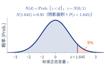
  • N(x) 表示均值为 0、标准差为 1 的标准正态分布随机变量小于 x 的概率: N(d)=Prob{z<d},z∼ϕ(0,1)
  • N(x) 的数值可以通过以下方式获取:
    • 使用 Excel 内置函数 NORMSDIST(或 NORM.S.DIST)
    • 查阅标准正态分布概率数值表
标准正态分布:N(1.645) ≈ 0.95 的阴影面积
  • 算例 – 线性插值法: 求 N(1.645) 的值?
    查表可得:N(1.64)=0.9495 以及 N(1.65)=0.9505,而 1.645 恰好位于两者中点:
    N(1.645)≈0.9495+0.5(0.9505−0.9495)=0.9500
    即标准正态变量小于 1.645 的概率约为 95%(构造置信区间时常用的分位数)。
Page 9 · Normal CDF & d1, d2Slide ↗

The Normal Cumulative Distribution Function (CDF)

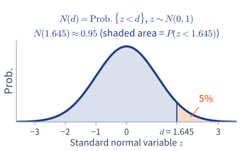
  • N(x) is the probability that a normally distributed variable with mean 0 and standard deviation 1 is less than x: N(d)=Prob{z<d},z∼ϕ(0,1)
  • Values of N(x) can be obtained by:
    • Using the Excel built-in function NORMSDIST (or NORM.S.DIST)
    • Looking up a standard normal probability table
Standard normal distribution: shaded area N(1.645) ≈ 0.95
  • Example – Linear Interpolation: What is N(1.645)?
    From the table: N(1.64)=0.9495 and N(1.65)=0.9505, and 1.645 lies exactly halfway between them:
    N(1.645)≈0.9495+0.5(0.9505−0.9495)=0.9500
    So the probability that a standard normal variable is less than 1.645 is about 95% (a quantile commonly used to construct confidence intervals).
第 10 页 · 正态分布累积函数幻灯片 ↗

Black-Scholes 模型的性质

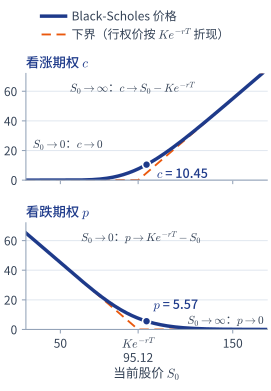
  • N(d1) 为期权的 Delta (Δ):衡量期权价格对基础资产价格微小变动的敏感度(Δcall=N(d1))。
  • N(d2):看涨期权最终被行权(ST>K)的风险中性概率。
  • 渐近边界行为:
    • 当 S0→∞ 时:c→S0−Ke−rT,且 p→0。
    • 当 S0→0 时:c→0,且 p→Ke−rT−S0。
Black-Scholes 看涨与看跌价格及其下界
Page 10 · Normal CDF & d1, d2Slide ↗

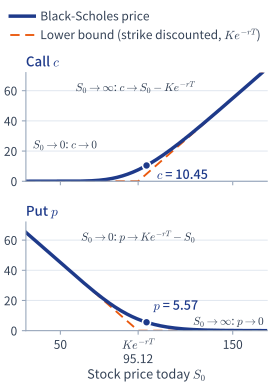
Properties of the Black-Scholes Model

  • N(d1) is the delta of the option: the sensitivity of option price to spot price changes (Δcall=N(d1)).
  • N(d2): The risk-neutral probability that the call option will be exercised (ST>K).
  • Asymptotic Behavior:
    • As S0→∞: c→S0−Ke−rT, and p→0.
    • As S0→0: c→0, and p→Ke−rT−S0.
Schematic of call and put prices against S0 with the lower bounds for S0 small and S0 large
第 11 页 · 正态分布累积函数幻灯片 ↗

无红利股票 Black-Scholes 完整估值算例

参数设定: S0=$100,K=$100,r=5%,σ=20%,T=1 年。股票不支付红利。

步骤 1:计算 d1,d2 及正态分布 CDF 值

ln⁡(100/100)=0,σT=0.2 (r+12σ2)T=0.05+0.02=0.07 d1=(0+0.07)/0.2=0.3500 d2=0.3500−0.2000=0.1500

标准正态累积分布函数值:

N(d1)=N(0.35)=0.6368 N(d2)=N(0.15)=0.5596 N(−d1)=1−0.6368=0.3632 N(−d2)=1−0.5596=0.4404

步骤 2:期权定价与买卖权平价检验

折现执行价格:Ke−rT=100e−0.05=$95.1229

c=100(0.6368)−95.1229(0.5596) c=63.68−53.23=$10.45 p=95.1229(0.4404)−100(0.3632) p=41.89−36.32=$5.57

CAmer=c=$10.45(无红利股票美式看涨期权永不应提前行权!)

买卖权平价定理检验:

c+Ke−rT=10.45+95.12=$105.57 p+S0=5.57+100.00=$105.57 ✓ 买卖权平价定理精确成立!

本例为简化算例;课本原题完整解答见《Hull 习题与解答》第 8 讲。

Page 11 · Normal CDF & d1, d2Slide ↗

Complete Black-Scholes Valuation Example: Non-Dividend-Paying Stock

Setup: S0=$100,K=$100,r=5%,σ=20%,T=1 year. The stock pays no dividends.

Step 1: Compute d1,d2 and Normal CDFs

ln⁡(100/100)=0,σT=0.2 (r+12σ2)T=0.05+0.02=0.07 d1=(0+0.07)/0.2=0.3500 d2=0.3500−0.2000=0.1500

Standard normal CDF values:

N(d1)=N(0.35)=0.6368 N(d2)=N(0.15)=0.5596 N(−d1)=1−0.6368=0.3632 N(−d2)=1−0.5596=0.4404

Step 2: Option Prices & Parity Check

Discounted strike: Ke−rT=100e−0.05=$95.1229

c=100(0.6368)−95.1229(0.5596) c=63.68−53.23=$10.45 p=95.1229(0.4404)−100(0.3632) p=41.89−36.32=$5.57

CAmer=c=$10.45 (an American call on a non-dividend-paying stock should never be exercised early!)

Put-Call Parity Check:

c+Ke−rT=10.45+95.12=$105.57 p+S0=5.57+100.00=$105.57 ✓ Put-call parity holds exactly!

This is a simplified example. Original Hull problem with full solution: see Hull Exercises & Solutions, Lecture 8.

第 12 页 · 正态分布累积函数幻灯片 ↗

交互实验:拖动股价,看 BS 价格怎么变

默认是上一页的算例(S0=K=100,r=5%,σ=20%,T=1 年):看涨 $10.45,看跌 $5.57。在四个页签里依次看 d1、d2 与平价检验、到期分布、隐含波动率的二分求解和希腊字母。 新窗口全屏打开 ↗

Page 12 · Normal CDF & d1, d2Slide ↗

Interactive Black-Scholes Explorer

The defaults are the previous page's example (S0=K=100, r=5%, σ=20%, T=1 year): call $10.45, put $5.57. Use the four tabs for d1, d2 and the parity check, the distribution of ST, implied volatility by bisection, and the Greeks. Open in New Window ↗

第 13 页 · 风险中性定价原理幻灯片 ↗

风险中性定价原理 (Risk-Neutral Valuation)

  • 变量 μ(股票预期收益率)并未出现在 Black-Scholes 公式中:
    • 投资者的风险偏好完全不影响期权理论价格!
  • Black-Scholes 公式独立于风险偏好的这一性质,使其与风险中性定价原理完全契合:
    • 在“风险中性”世界中,资产的初始价值等于其在到期日预期收益按无风险利率 r 进行折现的现值。
  • 当前资产价格:S0=e−rTE[ST]⟹E[ST]=S0erT
  • 远期合约(多头)当前价值(fT:合约在到期日 T 的价值):
    f0=e−rTE[fT]=e−rTE[FT−F0]=e−rTE[ST]−F0e−rT=e−rT⋅S0erT⏟E(ST)−F0e−rT=S0−F0e−rT=(FT−F0)e−rT
  • 看涨期权当前价值(cT=max(ST−K,0):期权在到期日 T 的回报):
    c0=e−rTE[cT]=e−rTE[max[ST−K,0]]=…Black-Scholes 公式
Page 13 · Risk-Neutral ValuationSlide ↗

Risk-Neutral Valuation

  • The variable μ does not feature in the Black-Scholes analysis:
    • The risk preferences of investors do not affect option prices!
  • The preference-independent nature of the Black-Scholes formula makes it consistent with the risk-neutral valuation principle:
    • In a “risk-neutral” world, the initial value of an asset is equal to its discounted expected payoff at maturity, discounted at r.
  • Current asset price: S0=e−rTE[ST]⟹E[ST]=S0erT
  • Current value of a (long) forward contract (fT: the contract's value at maturity T):
    f0=e−rTE[fT]=e−rTE[FT−F0]=e−rTE[ST]−F0e−rT=e−rT⋅S0erT⏟E(ST)−F0e−rT=S0−F0e−rT=(FT−F0)e−rT
  • Current value of a call option (cT=max(ST−K,0): the option payoff at maturity T):
    c0=e−rTE[cT]=e−rTE[max[ST−K,0]]=…Black-Scholes formula
第 14 页 · 历史波动率估算幻灯片 ↗

波动率的本质特征 (The Nature of Volatility)

  • 波动率产生的根源:
    • 在有效市场假说(EMH)下,波动率反映了新信息持续流入市场的过程。
    • 交易活动本身也会产生波动(市场微观结构效应、流动性冲击)。
  • 交易日 vs 日历日:
    • 市场开市交易时的资产波动率通常显著高于闭市期间(周末、节假日)。
    • 因此,在估算波动率和期权定价时,时间期限 T 通常以交易日(通常按每年 252 个交易日计算)而非日历日(365 天)进行折算计量。
Page 14 · Estimating VolatilitySlide ↗

The Nature of Volatility

  • Causes of volatility:
    • Under the Efficient Market Hypothesis (EMH), volatility represents new information arriving in the market.
    • Trading itself causes volatility (market microstructure, liquidity shocks).
  • Trading Days vs Calendar Days:
    • Volatility is usually much greater when the market is open (i.e. the asset is trading), than when it is closed (weekends, holidays).
    • For this reason, time T is usually measured in trading days (typically 252 days per year), not calendar days (365 days), for the purposes of estimating volatility and pricing options.
第 15 页 · 历史波动率估算幻灯片 ↗

利用历史数据估算波动率
(Hull,第 320–321 页)

  • 假设我们在时间间隔为 τ 年的时间点上拥有价格观测值 S0,S1,…,Sn(共 n+1 个价格)。
  • 定义第 i 期(i=1,…,n)的连续复利收益率(对数收益率):
    ui=ln⁡(SiSi−1)
  • 若 s 表示样本收益率 u1,u2,…,un 的样本标准差(u¯:这 n 个收益率的样本均值),则年化历史波动率的估计值为 σ^=s/τ:
    s=1n−1∑i=1n(ui−u¯)2
  • 历史波动率反映的是历史信息(向后看),并不总能作为未来波动率的可靠预测指标。
迷你算例: 连续 5 个交易日的收盘价(τ=1/252 年,共 n=4 个收益率;表中收益率以 % 计)
日 iSiui(%)(ui−u¯)2(%²)
0100——
199−1.00503.0415
21012.00011.5904
31020.98520.0606
41030.97560.0560
合计u¯=0.73904.7485
s=4.74854−1%=1.2581%(每个交易日) σ^=sτ=1.2581%×252≈19.97%
Page 15 · Estimating VolatilitySlide ↗

Estimating Volatility from Historical Data
(Hull, pages 320–321)

  • We observe S0,S1,…,Sn (n+1 prices) at intervals of τ years.
  • Define the continuously compounded return (log-return) for period i=1,…,n:
    ui=ln⁡(SiSi−1)
  • If s is the sample standard deviation of u1,u2,…,un (u¯: their sample mean), the annualized volatility estimate is σ^=s/τ:
    s=1n−1∑i=1n(ui−u¯)2
  • Historical volatility is backward-looking and may not reliably predict future volatility.
Mini Example: 5 consecutive daily closing prices (τ=1/252 year, n=4 returns; returns in %)
Day iSiui (%)(ui−u¯)2 (%²)
0100——
199−1.00503.0415
21012.00011.5904
31020.98520.0606
41030.97560.0560
Totalu¯=0.73904.7485
s=4.74854−1%=1.2581% (per trading day) σ^=sτ=1.2581%×252≈19.97%
第 16 页 · 历史波动率估算幻灯片 ↗

隐含波动率 (Implied Volatility)

  • 市场期权实际交易价格与隐含波动率之间存在严格的一一对应关系。
  • 期权的隐含波动率,是指使得 Black-Scholes 理论定价恰好等于市场上观察到的期权实际交易价格的波动率参数。
  • 计算隐含波动率需要对 Black-Scholes 公式进行反向求解(不存在解析求导的代数显式逆函数):
    • 数值迭代算法:试错法(Trial and error)、牛顿-拉夫逊法(Newton-Raphson)
    • Excel 单变量求解工具(数据 → 模拟分析 → 单变量求解)
迷你算例(接第 11 页): S0=K=$100,T=1,r=5% 的看涨期权市价为 $10.45。试错反解 σ:
试算 σBSM 价格 c与市价 $10.45 比较
10%$6.80太低
30%$14.23太高
20%$10.45正好 ✓
隐含波动率 σimpl=20%(正是第 11 页定价时使用的波动率!)
  • 隐含波动率的关键重要性:
    • 可用市场一致认可的波动率水平为缺乏流动性或场外(OTC)期权定价。
    • 交易员普遍以隐含波动率而非美元价格报价沟通。
    • 是前瞻性的市场预期指标(如著名的 VIX 指数)。
Page 16 · Estimating VolatilitySlide ↗

Implied Volatility

  • There is a one-to-one correspondence between market option prices and implied volatilities.
  • The implied volatility is the volatility for which the Black-Scholes price equals the observed market price.
  • Computing it requires inverting the Black-Scholes formula (no closed-form inverse):
    • Iterative numerical methods: Trial and error, Newton-Raphson
    • Excel's Goal Seek (Data → What-If Analysis → Goal Seek)
Mini Example (from page 11): A call with S0=K=$100,T=1,r=5% trades at $10.45. Trial and error for σ:
Trial σBSM price cvs market $10.45
10%$6.80Too low
30%$14.23Too high
20%$10.45Exact match ✓
Implied volatility σimpl=20% (the volatility used on page 11!)
  • The Importance of Implied Volatility:
    • Price illiquid or OTC options at market-consistent volatility.
    • Traders quote in implied volatility rather than dollar prices.
    • A forward-looking measure of market expectations (e.g. the VIX index).
第 17 页 · 红利与美式看涨期权幻灯片 ↗

红利对期权价格的影响

  • 对支付红利股票的欧式期权进行估值时,只需将 Black-Scholes 公式中的现货股票价格 S0 替换为扣除红利现值 PV(D)(D:红利金额)后的调整后股票价格:
    S0→S0∗=S0−PV(D)
    注意:此处仅需扣除在期权有效期内发生除息的红利现值。
  • 因此,支付红利股票的欧式看涨与看跌期权价格分别为:
    c=S0∗N(d1)−Ke−rTN(d2)(3)p=Ke−rTN(−d2)−S0∗N(−d1)(4)
    其中:
    d1=ln⁡(S0∗/K)+(r+σ2/2)TσTd2=ln⁡(S0∗/K)+(r−σ2/2)TσT=d1−σT
Page 17 · Dividends & American CallsSlide ↗

The Impact of Dividends on Option Prices

  • European options on dividend-paying stocks are valued by substituting into the Black-Scholes formula, the stock price S0 with the difference between the stock price and the present value PV(D) of the dividends (D: the dividend amount):
    S0→S0∗=S0−PV(D)
    Only dividends with ex-dividend dates during the life of the option should be included.
  • Thus the prices of a call and a put on a dividend-paying stock are:
    c=S0∗N(d1)−Ke−rTN(d2)(3)p=Ke−rTN(−d2)−S0∗N(−d1)(4)
    where:
    d1=ln⁡(S0∗/K)+(r+σ2/2)TσTd2=ln⁡(S0∗/K)+(r−σ2/2)TσT=d1−σT
第 18 页 · 红利与美式看涨期权幻灯片 ↗

美式看涨期权与看跌期权

  • 对于不支付红利的股票,美式看涨期权绝不应提前行权(C=c)。
  • 对于支付红利的股票,美式看涨期权仅在除息日即刻之前提前行权才可能最优。
  • 美式看跌期权在满足特定条件时(深度实值、利率较高),即使股票不支付红利,通常也应提前行权。
  • 美式看涨期权的价格可以通过两个欧式看涨期权价格的最大值进行近似估算(布莱克近似法 / Black's approximation):
    • 期权 1: 到期日与美式期权相同、股价扣除红利现值后的欧式看涨期权(即使用 S0∗=S0−PV(D),其中 D 为红利,PV(D) 为红利现值)。
    • 期权 2: 在最后一个除息日即刻前到期的欧式看涨期权(使用未经扣减的当前股价 S0)。
Page 18 · Dividends & American CallsSlide ↗

American Calls and Puts

  • An American call on a non-dividend-paying stock should never be exercised early (C=c).
  • An American call on a dividend-paying stock should only ever be exercised immediately prior to an ex-dividend date.
  • American puts are typically exercised early under the right conditions, even when the stock pays no dividends.
  • The price of the American call is estimated as the maximum of two European option prices (Black's approximation):
    • Option 1: The European call maturing at the same date as the American option (with S0∗=S0−PV(D), where D is the dividend and PV(D) its present value).
    • Option 2: The European call maturing just before the final ex-dividend date (with unadjusted S0).
第 19 页 · 红利与美式看涨期权幻灯片 ↗

离散红利 BSM 模型与美式看涨期权布莱克近似

参数设定: S0=$100,σ=20%,r=5%(与上面的算例相同)。预计 6 个月后(t1=0.5 年)支付红利 D=$5。看涨期权执行价格 K=$90(深度实值,提前行权才可能划算),期限 T=1 年。

部分 (a):欧式看涨期权 (c≈$12.93)

红利现值:PV(D)=5e−0.05×0.5=$4.8765。

调整后股票价格:S0∗=100−4.8765=$95.1235。

d1=[ln⁡(95.1235/90)+0.07]/0.2 d1=0.6268 d2=0.6268−0.2000=0.4268 N(d1)=0.7346,N(d2)=0.6652 c=95.1235(0.7346)−90e−0.05(0.6652) c≈69.88−56.95=$12.93

部分 (b):布莱克近似估算美式看涨期权 (C≈$13.50)

对比两只欧式看涨期权:

  • 期权 1(期限 T=1): 股票价格 S0∗=$95.1235⟹c1≈$12.93
  • 期权 2(期限 t1=0.5): 除息日前一刻到期,用未扣除红利的现价 S0=$100:
    d1=[ln⁡(100/90)+0.035]/(0.20.5)=0.9925 d2=0.9925−0.1414=0.8511 N(d1)=0.8395,N(d2)=0.8026 c2=100(0.8395)−90e−0.025(0.8026)≈$13.50
CAmer≈max(c1,c2)=$13.50
除息日即刻前(t1=6 个月)提前行权最优:c2≈$13.50>c1≈$12.93。提前行权立刻锁定 $5 红利,胜过保留剩余 6 个月的时间价值!课本原题完整解答见《Hull 习题与解答》第 8 讲。
Page 19 · Dividends & American CallsSlide ↗

Discrete-Dividend BSM & Black's Approximation for American Calls

Setup: S0=$100,σ=20%,r=5% (same as the worked example above). A dividend D=$5 is expected in 6 months (t1=0.5 year). Call strike K=$90 (deep in the money, so that early exercise can pay), maturity T=1 year.

Part (a): European Call (c≈$12.93)

PV of dividend: PV(D)=5e−0.05×0.5=$4.8765.

Adjusted stock price: S0∗=100−4.8765=$95.1235.

d1=[ln⁡(95.1235/90)+0.07]/0.2 d1=0.6268 d2=0.6268−0.2000=0.4268 N(d1)=0.7346,N(d2)=0.6652 c=95.1235(0.7346)−90e−0.05(0.6652) c≈69.88−56.95=$12.93

Part (b): Black's Approximation for the American Call (C≈$13.50)

Compare two European calls:

  • Option 1 (maturity T=1): Stock price S0∗=$95.1235⟹c1≈$12.93
  • Option 2 (maturity t1=0.5): Matures just before the ex-dividend date; use the unadjusted price S0=$100:
    d1=[ln⁡(100/90)+0.035]/(0.20.5)=0.9925 d2=0.9925−0.1414=0.8511 N(d1)=0.8395,N(d2)=0.8026 c2=100(0.8395)−90e−0.025(0.8026)≈$13.50
CAmer≈max(c1,c2)=$13.50
Exercising early, just before the ex-dividend date (t1=6 months) is optimal: c2≈$13.50>c1≈$12.93. Early exercise locks in the $5 dividend immediately, which beats keeping the remaining 6 months of time value! Original Hull problem with full solution: see Hull Exercises & Solutions, Lecture 8.