← 目录Index 第7讲:二叉树期权定价模型导论Lecture 7 · Introduction to Binomial Trees 幻灯片Slides
本讲目录Contents
  1. 学习目标Learning Objectives
  2. 单期二叉树模型One-Period Model
  3. 无套利复制组合No-Arbitrage Arguments
  4. 风险中性定价Risk-Neutral Valuation
  5. 确定u与d参数Determining u and d
  6. 两期二叉树模型Two-Step Trees
  7. 美式期权定价American Options
  8. 二叉树实务应用Trees in Practice
  9. 连续红利收益率Continuous Dividend Yield
第 1 页幻灯片 ↗
第 7 讲
二叉树期权定价模型导论
John C. Hull 第12章
每周提示
股票上涨的“风险中性”概率意味着其预期收益率等于无风险利率。这与真实世界中股票实际的上涨概率截然不同。
✦ UTS商学院
Page 1Slide ↗
Lecture 7
Introduction to Binomial Trees
Hull, Chapter 12
Tip of the week
The risk-neutral probability that the stock will go up, implies an expected return equal to the risk-free rate. It is different to the probability of an up movement in the real world.
✦ UTS Business School
第 2 页 · 学习目标幻灯片 ↗

学习目标

  • 利用单期二叉树模型对无红利股票的欧式看涨与看跌期权进行定价
  • 无套利分析原理:
    • 定义并计算期权的 Delta (Δ)
  • 风险中性定价:
    • 定义并计算风险中性概率
    • 比较真实世界(实际)概率与风险中性概率
  • 从观测到的市场数据中计算二叉树模型参数
  • 模型拓展应用:
    • 多期二叉树模型
    • 美式期权定价
    • 调整二叉树模型以处理连续红利收益率
Page 2 · Learning ObjectivesSlide ↗

Learning Objectives

  • Use the one-period binomial model to price European call and put options on a non-dividend paying stock
  • No-arbitrage arguments:
    • Define and compute delta of an option
  • Risk-neutral valuation:
    • Define and compute risk-neutral probabilities
    • Compare real-world (actual) and risk-neutral probabilities
  • Compute the parameters of a binomial model from observed market data
  • Extensions:
    • Multi-period binomial trees
    • Pricing of American options
    • Adjust the binomial model to cater for dividend yield
第 3 页 · 单期二叉树模型幻灯片 ↗

简单例子 – 单期二叉树模型

数字取最简单的:一年后股价要么涨 20% 要么跌 20%(相当于 σ=20%),利率为 0
  • 基础资产: 股票当前价格 S0=$100。一年后(T=1)股票价格只有两种可能: 上涨至 Su=$120 或 下跌至 Sd=$80(此处假定股价只有这两种走势;这里 u 为上涨因子、d 为下跌因子,Su=uS0,Sd=dS0,不同于前面讲中表示储存成本的 u)。
  • 待定价期权: 一年期看涨期权,执行价 K=$100,无风险利率 r=0。
    • 状态 u(上涨):到期回报 fu=max[Su−K,0]=max[120−100,0]=$20
    • 状态 d(下跌):到期回报 fd=max[Sd−K,0]=max[80−100,0]=$0
单期股票价格与期权回报二叉树
上涨 (u = 1.20) 下跌 (d = 0.80) S₀ = $100 f₀ = ? Su = $120 fu = $20 Sd = $80 fd = $0
问题:这份看涨期权今天值多少钱(f0=?)?下一页用无套利组合算出来。
Page 3 · One-Period ModelSlide ↗

Simple Example – One-Period Binomial Model

The simplest numbers: in one year the stock rises 20% or falls 20% (σ=20%), and the interest rate is 0
  • Underlying asset: the current stock price is S0=$100. In one year (T=1) the stock price has only two possible values: up to Su=$120 or down to Sd=$80 (assumed behaviour; here u,d are the up and down factors: Su=uS0, Sd=dS0).
  • Option to price: a one-year call option with strike K=$100; the risk-free rate is r=0.
    • State u (up): terminal payoff fu=max[Su−K,0]=max[120−100,0]=$20
    • State d (down): terminal payoff fd=max[Sd−K,0]=max[80−100,0]=$0
One-Step Stock Price and Option Payoff Tree
Up (u = 1.20) Down (d = 0.80) S₀ = $100 f₀ = ? Su = $120 fu = $20 Sd = $80 fd = $0
Question: what is this call option worth today (f0=?)? The next page works it out with a no-arbitrage portfolio.
第 4 页 · 无套利复制组合幻灯片 ↗

简单例子 – 无套利分析原理

接上一页:S0=$100,一年后涨到 $120 或跌到 $80;K=$100 看涨期权
  • 考虑由以下资产构成的投资组合:
    • 买入 Δ 股股票,以及
    • 卖出 1 份看涨期权空头
  • 到期时投资组合的价值为 (Δ×ST)−fT(ST 为股票在到期日 T 的价格,fT 为期权在到期日 T 的回报):
    • 若股票上涨,组合价值为 (Δ×$120)−$20
    • 若股票下跌,组合价值为 (Δ×$80)−$0
  • 当两种状态下的到期支付完全相等时,该投资组合即为无风险组合:
    (Δ×$120)−$20=(Δ×$80)−$0
    由此可解得:
    Δ=$20−$0$120−$80=2040=0.5
  • Δ 代表期权价格变动与股票价格变动的比率(对冲比率)。
Page 4 · No-Arbitrage ArgumentsSlide ↗

Simple Example – No-Arbitrage Arguments

Continued: S0=$100, up to $120 or down to $80 in one year; K=$100 call
  • Consider a portfolio consisting of:
    • a long position in Δ units of the asset, and
    • a short position in 1 call option
  • The portfolio value at maturity is (Δ×ST)−fT (where ST is the stock price and fT the option payoff at maturity T):
    • If the stock rises: (Δ×$120)−$20
    • If the stock falls: (Δ×$80)−$0
  • The portfolio is riskless when the two state payoffs are equal:
    (Δ×$120)−$20=(Δ×$80)−$0
    which gives:
    Δ=$20−$0$120−$80=2040=0.5
  • Δ is the change in the option price over the change in the stock price (the hedge ratio).
第 5 页 · 无套利复制组合幻灯片 ↗

简单例子 – 无套利分析原理

接上一页:Δ=0.5,利率为 0 不需要折现
  • 现在代入 Δ=0.5 计算投资组合的到期价值:
    • 若股票上涨,价值为 (0.5×$120)−$20=$60−$20=$40
    • 若股票下跌,价值为 (0.5×$80)−$0=$40
  • 两种状态下结果完全一样,该投资组合是完全无风险的。由于利率为 0(e−rT=e0=1),现值无需折现:
    $40e−0×1=$40
  • 投资组合的期初价值为:
    (Δ×S0)−f0=$40
    由此推导得出:
    f0=(0.5×$100)−$40=$50−$40=$10
这份看涨期权今天值 $10。课本原题多了 12% 的连续复利,只需多一步折现,步骤完全一样,完整解答见《Hull 习题与解答》第 7 讲。
Page 5 · No-Arbitrage ArgumentsSlide ↗

Simple Example – No-Arbitrage Arguments

Continued: Δ=0.5; with an interest rate of 0, no discounting is needed
  • Substituting Δ=0.5, the terminal portfolio value is:
    • If the stock rises: (0.5×$120)−$20=$60−$20=$40
    • If the stock falls: (0.5×$80)−$0=$40
  • Identical in both states — the portfolio is completely risk-free. With rate 0 (e−rT=e0=1) there is no discounting:
    $40e−0×1=$40
  • The initial portfolio value is:
    (Δ×S0)−f0=$40
    from which it follows that:
    f0=(0.5×$100)−$40=$50−$40=$10
This call is worth $10 today. The textbook original adds 12% continuous compounding — one extra discounting step, otherwise identical. Original Hull problem with full solution: see Hull Exercises & Solutions, Lecture 7.
第 6 页 · 无套利复制组合幻灯片 ↗

一般情况下的无套利分析

  • 股票初始价格为 S0,到期价格要么为 ST=Su=uS0,要么为 ST=Sd=dS0:
    • 若 ST=uS0,则衍生品到期回报 fu 确定已知。
    • 若 ST=dS0,则衍生品到期回报 fd 确定已知。
S0f0 = ?Su = uS0fuSd = dS0fd
  • 构建如下投资组合:
    • 买入 Δ 股股票,以及
    • 卖出 1 份衍生期权空头
  • 到期时投资组合的价值为 uS0Δ−fu 或 dS0Δ−fd。
  • 当投资组合满足以下条件时实现完全无风险:
    uS0Δ−fu=dS0Δ−fd
    由此可推导解得:
    Δ=fu−fduS0−dS0=fu−fdSu−Sd
Page 6 · No-Arbitrage ArgumentsSlide ↗

No-Arbitrage Arguments in General

  • Initial stock price is S0, and ST=Su=uS0 or ST=Sd=dS0:
    • If ST=uS0, then the derivative payoff fu is known.
    • If ST=dS0, then the derivative payoff fd is known.
S0f0 = ?Su = uS0fuSd = dS0fd
  • Consider the portfolio consisting of:
    • a long position in Δ units of the asset, AND
    • a short position in one option
  • The value of the portfolio at maturity is uS0Δ−fu or dS0Δ−fd.
  • The portfolio is riskless when:
    uS0Δ−fu=dS0Δ−fd
    from which it follows that:
    Δ=fu−fduS0−dS0=fu−fdSu−Sd
第 7 页 · 无套利复制组合幻灯片 ↗

一般情况下的无套利分析

  • 投资组合的到期终值为 uS0Δ−fu=dS0Δ−fd。
  • 投资组合的初始价值:
    • 由于最终组合价值与市场涨跌方向完全无关,该组合是无风险的,因此: (uS0Δ−fu)e−rT=(dS0Δ−fd)e−rT
    • 今日构建该投资组合的成本为:ΔS0−f0
  • 将上述两种表达式联立等置:
    f0=ΔS0−(uS0Δ−fu)e−rT=ΔS0−(dS0Δ−fd)e−rT
  • 代入 Δ 的表达式并进行代数化简可得:
    f0=e−rT[pfu+(1−p)fd]其中p=erT−du−d
    这里 p 表示股价上涨的风险中性概率(第 5 讲中 p 曾表示看跌期权价格,此处含义不同)。
Page 7 · No-Arbitrage ArgumentsSlide ↗

No-Arbitrage Arguments in General

  • The terminal value of the portfolio is uS0Δ−fu=dS0Δ−fd.
  • The initial value of the portfolio:
    • Since the final portfolio value is independent of the market direction, the portfolio is risk-free, thus: (uS0Δ−fu)e−rT=(dS0Δ−fd)e−rT
    • The cost to set up the portfolio today is: ΔS0−f0
  • Thus by equating these two representations:
    f0=ΔS0−(uS0Δ−fu)e−rT=ΔS0−(dS0Δ−fd)e−rT
  • By substituting Δ and simplifying algebraically:
    f0=e−rT[pfu+(1−p)fd]withp=erT−du−d
    Here p is the risk-neutral probability of an up move (in Lecture 5 p was the put price; this is a new meaning).
第 8 页 · 风险中性定价幻灯片 ↗

“风险中性”概率

  • 风险中性投资者认为所有资产价格均以无风险利率 r 增长,因此在对未来所有现金流估值时均以 r 进行折现。
  • 在“风险中性”世界中:
    • 所有资产的预期收益率都等于无风险利率 r
    • 资产的期初现值等于其到期预期回报以无风险利率贴现后的数值
p1 − pS0f0 = ?Su = uS0fuSd = dS0fd
  • 股票上涨的“风险中性”概率 p 满足(E[⋅] 表示在风险中性概率下的期望值):
    E[ST]=S0erT⟹S0=e−rTE[ST]=e−rT[pSu+(1−p)Sd]
  • 真实世界(实际)中股票上涨的概率 pa 与风险中性概率 p 存在本质差异。
    • 若资产的实际预期收益率为 μ,则(Ea[⋅] 表示在真实世界概率 pa 下的期望值): S0=e−μTEa[ST]=e−μT[paSu+(1−pa)Sd]
Page 8 · Risk-Neutral ValuationSlide ↗

The “Risk-Neutral” Probability

  • Risk-neutral investors believe that asset prices grow at the risk-free rate r and thus value all future cash-flows by discounting at r.
  • In a “risk-neutral” world:
    • the expected return of every asset is the risk-free rate r
    • the initial value of an asset is equal to its expected payoff at maturity, discounted at the risk-free rate
p1 − pS0f0 = ?Su = uS0fuSd = dS0fd
  • The “risk-neutral” probability p of an up movement satisfies (E[⋅] is the expected value under the risk-neutral probabilities):
    E[ST]=S0erT⟹S0=e−rTE[ST]=e−rT[pSu+(1−p)Sd]
  • The real-world (actual) probability pa of stock going up is different to the risk-neutral probability p.
    • When μ is the expected return on the asset, then (Ea[⋅] is the expected value under the actual real-world probabilities pa): S0=e−μTEa[ST]=e−μT[paSu+(1−pa)Sd]
第 9 页 · 风险中性定价幻灯片 ↗

简单例子 – 风险中性定价

同一个例子:S0=$100,一年后 $120 或 $80;K=$100 看涨期权,r=0
  • 设 p 为股票上涨的“风险中性”概率,则有:
    E[ST]=S0erT⟹pSu+(1−p)Sd=S0erT(1) E[fT]=f0erT⟹pfu+(1−p)fd=f0erT(2)
p1 − pS0 = $100f0 = ?Su = $120fu = $20Sd = $80fd = $0
  • 由方程 (1) 代入已知数据 S0=100,Su=120,Sd=80,r=0,T=1(注意 e0=1):
    $120p+$80(1−p)=$100 p=$100−$80$120−$80=2040=0.5
  • 由方程 (2) 可得期权价值(fu=$20,fd=$0):
    f0=e−rT[pfu+(1−p)fd] =e0[(0.5×$20)+(0.5×$0)]=$10+$0=$10
与无套利组合算出的 $10 完全相同 —— 风险中性定价只是换了个算法:先求概率 p,再对预期回报折现。
Page 9 · Risk-Neutral ValuationSlide ↗

Simple Example – Risk-Neutral Valuation

Same example: S0=$100, $120 or $80 in one year; K=$100 call, r=0
  • Let p be the “risk-neutral” probability of an up move; then:
    E[ST]=S0erT⟹pSu+(1−p)Sd=S0erT(1) E[fT]=f0erT⟹pfu+(1−p)fd=f0erT(2)
p1 − pS0 = $100f0 = ?Su = $120fu = $20Sd = $80fd = $0
  • Substituting S0=100,Su=120,Sd=80,r=0,T=1 into equation (1) (note e0=1):
    $120p+$80(1−p)=$100 p=$100−$80$120−$80=2040=0.5
  • Equation (2) gives the option value (fu=$20,fd=$0):
    f0=e−rT[pfu+(1−p)fd] =e0[(0.5×$20)+(0.5×$0)]=$10+$0=$10
The same $10 as the no-arbitrage portfolio — risk-neutral valuation just solves for the probability p first, then discounts the expected payoff.
第 10 页 · 风险中性定价幻灯片 ↗

一般情况下的风险中性定价

  • 设 p 为股票上涨的“风险中性”概率: Su=uS0(p)Sd=dS0(1−p)
p1 − pS0f0 = ?Su = uS0fuSd = dS0fd
  • 在“风险中性”世界中,资产的初始价值等于其到期预期回报按无风险利率 r 折现的现值:
    E[ST]=S0erT⟹pSu+(1−p)Sd=S0erT(3) E[fT]=f0erT⟹pfu+(1−p)fd=f0erT(4)
  • 从方程 (3) 中解出 p:
    puS0+(1−p)dS0=S0erT⟹p=erT−du−d
  • 从方程 (4) 导出通用期权定价公式:
    f0=e−rT[pfu+(1−p)fd]
Page 10 · Risk-Neutral ValuationSlide ↗

Risk-Neutral Valuation in General

  • Let p be the “risk-neutral” probability of an up movement: Su=uS0(p)Sd=dS0(1−p)
p1 − pS0f0 = ?Su = uS0fuSd = dS0fd
  • In a “risk-neutral” world, the initial value of an asset is equal to its discounted expected payoff at maturity, discounted at r:
    E[ST]=S0erT⟹pSu+(1−p)Sd=S0erT(3) E[fT]=f0erT⟹pfu+(1−p)fd=f0erT(4)
  • From (3) we solve for p:
    puS0+(1−p)dS0=S0erT⟹p=erT−du−d
  • From (4) the general pricing formula is:
    f0=e−rT[pfu+(1−p)fd]
第 11 页 · 风险中性定价幻灯片 ↗

单步欧式看跌期权:无套利复制 vs 风险中性期望

同样取最简单的数字:利率为 0

设定: S0=$100,一年后(T=1)Su=$120,Sd=$80。利率 r=0。求 K=$100 看跌期权今天的价格 p0(p0 是期权价格,不是概率 p)。

方法一:复制组合 / Delta对冲

回报:fu=max[100−120,0]=0,fd=max[100−80,0]=$20。

Δ=fu−fdSu−Sd=0−20120−80=−0.5

卖出1份看跌期权 + 卖空0.5股股票(该组合的价值记为 Π;PV(⋅) 表示现值):

  • 上涨:−0.5(120)−0=−$60
  • 下跌:−0.5(80)−20=−$60
PV(Π)=−$60(r=0,无需折现) −0.5(100)−p0=−60⟹p0=$10

方法二:风险中性定价

u=1.20,d=0.80,erT=e0=1。

p=erT−du−d=1−0.801.20−0.80=0.200.40=0.5 1−p=0.5

折现风险中性预期回报:

p0=e0[0.5($0)+0.5($20)] =0+$10=$10

✓ 两种方法完全等价:p0=$10

Page 11 · Risk-Neutral ValuationSlide ↗

One-Step European Put: No-Arbitrage Replication vs Risk-Neutral Expectation

The same simplest-possible numbers: the interest rate is 0

Setup: S0=$100; in one year (T=1), Su=$120, Sd=$80. Interest rate r=0. Value the K=$100 put option, whose price today is p0 (an option price, not the probability p).

Method One: Replication / Delta Hedge

Payoffs: fu=max[100−120,0]=0, fd=max[100−80,0]=$20.

Δ=fu−fdSu−Sd=0−20120−80=−0.5

Sell 1 put + short 0.5 shares (portfolio value Π; PV(⋅) is present value):

  • Up: −0.5(120)−0=−$60
  • Down: −0.5(80)−20=−$60
PV(Π)=−$60(r=0; no discounting) −0.5(100)−p0=−60⟹p0=$10

Method Two: Risk-Neutral Pricing

u=1.20, d=0.80, erT=e0=1.

p=erT−du−d=1−0.801.20−0.80=0.200.40=0.5 1−p=0.5

Discount the risk-neutral expected payoff:

p0=e0[0.5($0)+0.5($20)] =0+$10=$10

✓ The two methods are exactly equivalent: p0=$10

第 12 页 · 确定u与d参数幻灯片 ↗

确定参数 u 与 d

  • 在实务中,通常采用 Cox, Ross and Rubinstein (1979) 的方法,根据资产价格波动率 σ 来校准确定 u 与 d。对于极小时间步长 Δt:
    u=eσΔt d=1u=e−σΔt
  • 示例:取 σ=20%,把 1 年分成两期,每期 Δt=0.5 年:
    u=eσΔt=e0.20.5=e0.1414=1.1519 d=1u=11.1519=0.8681
  • 下面的两期二叉树就用这组 u,d。前面单期例子里的 $120 / $80 是为了计算简单而直接给定的涨跌(±20%,相当于 σ=20%),并非由 CRR 公式算出。
Page 12 · Determining u and dSlide ↗

Determining u and d

  • In practice, u and d are usually calibrated from the asset price volatility σ using the Cox, Ross and Rubinstein (1979) approach. For a small time step Δt:
    u=eσΔt d=1u=e−σΔt
  • Example: take σ=20% and split the year into two steps of Δt=0.5 year:
    u=eσΔt=e0.20.5=e0.1414=1.1519 d=1u=11.1519=0.8681
  • The two-step tree on the next pages uses this u,d. The $120 / $80 in the one-step examples were given moves (±20%, i.e. σ=20%), not computed from the CRR formula.
第 13 页 · 两期二叉树模型幻灯片 ↗

简单例子 – 两期二叉树模型 (基础参数)

按上一页的 CRR 方法校准:σ=20%,每期半年;这一棵树下几页反复使用
市场参数与步长划分

S0=$100,r=5%(连续复利)
总到期时间 T=1 年,分两期,每期步长 Δt=0.5 年

涨跌因子与风险中性概率

u=eσΔt=e0.1414=1.1519,d=1u=e−σΔt=0.8681
p=erΔt−du−d=e0.05×0.5−0.86811.1519−0.8681=1.0253−0.86810.2838=0.5539
1−p=0.4461

股票价格两期演变二叉树 (Δt=0.5 年)
$100 t = 0 $115.19 $86.81 t = 0.5 年 $132.69 $100 $75.36 t = 1 年

每期贴现因子 e−0.05×0.5=0.9753。课本原题由 σ=22.9% 校准 u,d,完整解答见《Hull 习题与解答》第 7 讲。

Page 13 · Two-Step TreesSlide ↗

Simple Example – Two-Step Binomial Model (Parameters)

Calibrated by CRR as on the previous page: σ=20%, half a year per step; reused on later pages
Parameters & Step Size

S0=$100, r=5% (continuous compounding)
Maturity T=1 year; two steps of Δt=0.5 year

Factors & Risk-Neutral Probability

u=eσΔt=e0.1414=1.1519,d=1u=e−σΔt=0.8681
p=erΔt−du−d=e0.05×0.5−0.86811.1519−0.8681=1.0253−0.86810.2838=0.5539
1−p=0.4461

Two-Step Stock Price Evolution Tree (Δt=0.5 Years)
$100 t = 0 $115.19 $86.81 t = 0.5 Years $132.69 $100 $75.36 t = 1 Year

Per-step discount factor e−0.05×0.5=0.9753. The textbook original calibrates u,d from σ=22.9%. Original Hull problem with full solution: see Hull Exercises & Solutions, Lecture 7.

第 14 页 · 两期二叉树模型幻灯片 ↗

简单例子 – 两期二叉树模型 (看涨期权)

同一棵树:S0=$100,u=1.1519,d=0.8681,p=0.5539,每期贴现因子 0.9753

对执行价格 K=$100、到期时间 T=1 年的看涨期权进行定价(下面的 fu、fd 是半年末上涨、下跌节点处的期权价值,不再是到期回报):

到期看涨期权回报:

fuu=max[132.69−100,0]=32.69 fud=max[100−100,0]=0 fdd=max[75.36−100,0]=0

倒推逆向折现 (p=0.5539):

fu=e−0.025(0.5539×32.69+0.4461×0)=17.66 fd=e−0.025(0.5539×0+0.4461×0)=0 f0=e−0.025(0.5539×17.66+0.4461×0)=9.54

一年期欧式看涨期权的价格为 $9.54。

股票价格树$100$115.19$86.81$132.69$100$75.36期权价值树f0 = 9.54fu = 17.66fd = 0fuu = 32.69fud = 0fdd = 0
Page 14 · Two-Step TreesSlide ↗

Simple Example – Two-Step Binomial Tree (Call)

Same tree: S0=$100, u=1.1519, d=0.8681, p=0.5539, per-step discount factor 0.9753

Price a call option with strike K=$100 and maturity T=1 year (below, fu and fd are the option values at the up and down nodes after six months, no longer terminal payoffs):

Terminal call payoffs:

fuu=max[132.69−100,0]=32.69 fud=max[100−100,0]=0 fdd=max[75.36−100,0]=0

Backward induction (p=0.5539):

fu=e−0.025(0.5539×32.69+0.4461×0)=17.66 fd=e−0.025(0.5539×0+0.4461×0)=0 f0=e−0.025(0.5539×17.66+0.4461×0)=9.54

The price of the one-year European call option is $9.54.

Stock price tree$100$115.19$86.81$132.69$100$75.36Option value treef0 = 9.54fu = 17.66fd = 0fuu = 32.69fud = 0fdd = 0
第 15 页 · 两期二叉树模型幻灯片 ↗

简单例子 – 两期二叉树模型 (看跌期权)

同一棵树:S0=$100,u=1.1519,d=0.8681,p=0.5539,每期贴现因子 0.9753

对执行价格 K=$100、到期时间 T=1 年的看跌期权进行定价:

到期看跌期权回报:

fuu=max[100−132.69,0]=0 fud=max[100−100,0]=0 fdd=max[100−75.36,0]=24.64

倒推逆向折现 (p=0.5539):

fu=e−0.025(0.5539×0+0.4461×0)=0 fd=e−0.025(0.5539×0+0.4461×24.64)=10.72 f0=e−0.025(0.5539×0+0.4461×10.72)=4.66

一年期欧式看跌期权的价格为 $4.66。

股票价格树$100$115.19$86.81$132.69$100$75.36期权价值树f0 = 4.66fu = 0fd = 10.72fuu = 0fud = 0fdd = 24.64
Page 15 · Two-Step TreesSlide ↗

Simple Example – Two-Step Binomial Tree (Put)

Same tree: S0=$100, u=1.1519, d=0.8681, p=0.5539, per-step discount factor 0.9753

Price a put option with strike K=$100 and maturity T=1 year:

Terminal put payoffs:

fuu=max[100−132.69,0]=0 fud=max[100−100,0]=0 fdd=max[100−75.36,0]=24.64

Backward induction (p=0.5539):

fu=e−0.025(0.5539×0+0.4461×0)=0 fd=e−0.025(0.5539×0+0.4461×24.64)=10.72 f0=e−0.025(0.5539×0+0.4461×10.72)=4.66

The price of the one-year European put option is $4.66.

Stock price tree$100$115.19$86.81$132.69$100$75.36Option value treef0 = 4.66fu = 0fd = 10.72fuu = 0fud = 0fdd = 24.64
第 16 页 · 美式期权定价幻灯片 ↗

用计算器演示两期树与美式期权

打开即为前几页的两期树(S0=100,K=100,T=1,r=5%,σ=20%)。选 Put,再把 Tree values 改为 American,就是下一页的美式看跌期权。 新窗口全屏打开 ↗

Page 16 · American OptionsSlide ↗

Calculator Demo: American Put

Opens with the two-step tree of the previous pages (S0=100,K=100,T=1,r=5%,σ=20%). Choose Put and set Tree values to American for the American put on the next page. Open in New Window ↗

第 17 页 · 美式期权定价幻灯片 ↗

简单例子 – 两期二叉树模型 (美式看跌期权)

同一棵树,但利率为正(r=5%)时提前行权可能更划算

对执行价格 K=$100、到期时间 T=1 年的美式看跌期权进行定价:

  • 在每个节点检验提前行权是否为最优决策,即将对应的欧式期权价值(继续持有价值)与内在价值 max[K−St,0](St 为该节点的股票价格)进行比较:
fd=max[0.9753(0.5539×0+0.4461×24.64),100−86.81] =max[10.72,13.19]=13.19 fu=max[0.9753(0.5539×0+0.4461×0),0]=max[0,0]=0 f0=max[0.9753(0.5539×0+0.4461×13.19),0]=max[5.74,0]=5.74
  • 在节点 d(该节点股价 S=$86.81)处,提前行权为最优决策!立即行权拿到 $13.19>$10.72(继续持有的价值)。
  • 美式看跌期权价格为 $5.74,高于对应的欧式看跌期权价格 $4.66,提前行权溢价为 5.74−4.66=$1.08。
股票价格树$100$115.19$86.81$132.69$100$75.36期权价值树f0 = 5.74fu = 0fd = 13.19fuu = 0fud = 0fdd = 24.64提前行权
Page 17 · American OptionsSlide ↗

Simple Example – Two-Step Binomial Tree (American Put)

Same tree, but with a positive interest rate (r=5%), early exercise may be worthwhile
  • American put, K=$100, T=1 year. At each node compare the continuation value with the intrinsic value max[K−St,0] (St is the stock price at that node):
fd=max[0.9753(0.5539×0+0.4461×24.64),100−86.81] =max[10.72,13.19]=13.19 fu=max[0.9753(0.5539×0+0.4461×0),0]=max[0,0]=0 f0=max[0.9753(0.5539×0+0.4461×13.19),0]=max[5.74,0]=5.74
  • At node d (stock price S=$86.81 there) early exercise is optimal! Exercising now gives $13.19>$10.72 (continuation value).
  • The American put is worth $5.74, more than the corresponding European put at $4.66; the early-exercise premium is 5.74−4.66=$1.08.
Stock price tree$100$115.19$86.81$132.69$100$75.36Option value treef0 = 5.74fu = 0fd = 13.19fuu = 0fud = 0fdd = 24.64exercise early
第 18 页 · 美式期权定价幻灯片 ↗

两期二叉树:节点 d 处的提前行权决策

设定:与前几页完全相同的两期树:S0=$100,u=1.1519,d=0.8681,r=5%,Δt=0.5。
p=0.5539,1−p=0.4461,每期贴现因子 e−0.025=0.9753。
现在只换一个更深的行权价:看跌期权 K=$110。

第 (a) 部分:欧式看跌期权今天的价格 p0=$11.26

到期回报:puu=0,pud=110−100=10,pdd=110−75.36=34.64;pu、pd 为节点 u、d 处的看跌期权价值(不是概率 p)。

pu=0.9753[0.5539(0)+0.4461(10)]=4.35 pd=0.9753[0.5539(10)+0.4461(34.64)]=20.47 p0=0.9753[0.5539(4.35)+0.4461(20.47)] =$11.26

第 (b) 部分:美式看跌期权 P0=$12.44

逐节点提前行权检验:

  • 节点 u:内在价值 max[110−115.19,0]=0≤4.35⟹ 继续持有!价值 = $4.35
  • 节点 d:内在价值 110−86.81=23.19>20.47⟹ 提前行权!价值 = $23.19
  • 节点 0:继续持有价值 0.9753[0.5539(4.35)+0.4461(23.19)] =12.44。内在价值 110−100=10≤12.44⟹ 继续持有!价值 = $12.44
提前行权溢价为 $12.44−$11.26=$1.18(K=$100 时为 $1.08)。行权价越高、实值越深,在节点 d 处“立即拿钱走人”越划算:既避免了折现损失($23.19 今天拿比半年后期望值更值钱),又不必担心股价反弹回升。
Page 18 · American OptionsSlide ↗

Two-Step Binomial Tree: Early-Exercise Decision at Node d

Setup: exactly the same two-step tree as the previous pages: S0=$100, u=1.1519, d=0.8681, r=5%, Δt=0.5.
p=0.5539, 1−p=0.4461, per-step discount factor e−0.025=0.9753.
Now change only one thing — a higher strike: a put option with K=$110.

Part (a): European Put price today p0=$11.26

Terminal payoffs: puu=0, pud=110−100=10, pdd=110−75.36=34.64; pu, pd are put values at nodes u, d (not probabilities p).

pu=0.9753[0.5539(0)+0.4461(10)]=4.35 pd=0.9753[0.5539(10)+0.4461(34.64)]=20.47 p0=0.9753[0.5539(4.35)+0.4461(20.47)] =$11.26

Part (b): American Put P0=$12.44

Node-by-node early-exercise test:

  • Node u: intrinsic value max[110−115.19,0]=0≤4.35⟹ keep holding! Value = $4.35
  • Node d: intrinsic value 110−86.81=23.19>20.47⟹ EXERCISE EARLY! Value = $23.19
  • Node 0: continuation value 0.9753[0.5539(4.35)+0.4461(23.19)] =12.44. Intrinsic value 110−100=10≤12.44⟹ keep holding! Value = $12.44
The early-exercise premium is $12.44−$11.26=$1.18 ($1.08 when K=$100). The higher the strike and the deeper in the money, the better it is to “take the money and run” at node d: it avoids the discounting loss ($23.19 in hand today is worth more than an expected value six months away) and removes any worry about the stock price rebounding.
第 19 页 · 二叉树实务应用幻灯片 ↗

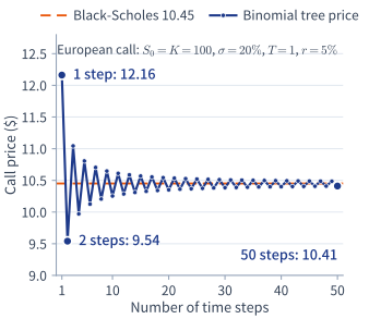
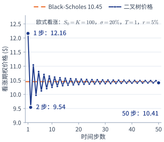
二叉树模型的实务应用

二叉树期权价格随步数收敛于 Black-Scholes 价格
  • 在实务中应用二叉树模型时,通常将期权的存续期划分为30步或更多时间步长。
  • 随着步数不断增加,离散二叉树计算出的期权价格将收敛于连续时间下的 Black-Scholes-Merton 理论解析解。
  • 二叉树模型能够非常便捷地扩展并处理离散分红付息。
Page 19 · Trees in PracticeSlide ↗

Binomial Trees in Practice

Binomial tree option price convergence versus number of steps
  • When the binomial model is used in practice the life of the option is typically divided into 30 or more time steps.
  • As the number of steps increases, the discrete tree price converges to the continuous Black-Scholes-Merton price.
  • Binomial trees are easily adapted to handle discrete dividend payments.
第 20 页 · 连续红利收益率幻灯片 ↗

风险中性定价 – 连续红利收益率

p1 − pS0f0 = ?Su = uS0fuSd = dS0fd
  • 在“风险中性”世界中,支付连续复利红利收益率 q 的股票预期收益率为 r−q。因此:
    E[ST]=S0e(r−q)T⟹pSu+(1−p)Sd=S0e(r−q)T(5) E[fT]=f0erT⟹pfu+(1−p)fd=f0erT(6)
  • 由方程 (5) 可推导出:
    puS0+(1−p)dS0=S0e(r−q)T⟹p=e(r−q)T−du−d
  • 由方程 (6) 将预期到期回报按无风险利率 r 折现:
    f0=e−rT[pfu+(1−p)fd]
Page 20 · Continuous Dividend YieldSlide ↗

Risk-Neutral Valuation – Dividend Yield

p1 − pS0f0 = ?Su = uS0fuSd = dS0fd
  • In a “risk-neutral” world, the expected return on a stock paying a continuously compounded dividend yield q is r−q. Thus:
    E[ST]=S0e(r−q)T⟹pSu+(1−p)Sd=S0e(r−q)T(5) E[fT]=f0erT⟹pfu+(1−p)fd=f0erT(6)
  • From (5) we have that:
    puS0+(1−p)dS0=S0e(r−q)T⟹p=e(r−q)T−du−d
  • From (6) we discount the expected payoff at r:
    f0=e−rT[pfu+(1−p)fd]
第 21 页 · 连续红利收益率幻灯片 ↗

简单例子 – 无套利分析原理
(支付红利股票的看跌期权)

股票每年派 2% 连续红利,所以持股数量会以 eqT 增长
  • 某股票当前价格为$100,一年后(T=1)其价格要么为$122.14,要么为$81.87(按第 11 页的 CRR 公式,σ=20%、Δt=1:u=e0.2=1.2214,d=1/u=0.8187)。
  • 对一年期看跌期权定价,已知 K=$100,q=2%,r=5%(均为连续复利):
    • 若 ST=Su=$122.14,则 fu=max[100−122.14,0]=$0
    • 若 ST=Sd=$81.87,则 fd=max[100−81.87,0]=$18.13
S0 = $100f0 = ?Su = $122.14fu = $0Sd = $81.87fd = $18.13
  • 构建由以下头寸组成的投资组合:
    • 买入 Δ 股股票,以及
    • 卖出 1 份看跌期权空头
  • 红利再投资使持股数量增长为原来的 eqT=e0.02×1=e0.02 倍,到期时组合价值为 (Δ×STeqT)−fT:
    • 若股票上涨:(Δ×$122.14e0.02)−$0
    • 若股票下跌:(Δ×$81.87e0.02)−$18.13
下一页解出 Δ 和期权价格。课本原题(3 个月期、q=3%,r=12%)完整解答见《Hull 习题与解答》第 7 讲。
Page 21 · Continuous Dividend YieldSlide ↗

Simple Example – No-Arbitrage Arguments
(Put on a Dividend-Paying Stock)

A 2% continuous dividend yield means the number of shares held grows by a factor of eqT
  • A stock is currently $100; in one year (T=1) it will be $122.14 or $81.87 (from the CRR formula of page 11 with σ=20%, Δt=1: u=e0.2=1.2214,d=1/u=0.8187).
  • Price a one-year put with K=$100,q=2%,r=5% (both continuously compounded):
    • If ST=Su=$122.14, then fu=max[100−122.14,0]=$0
    • If ST=Sd=$81.87, then fd=max[100−81.87,0]=$18.13
S0 = $100f0 = ?Su = $122.14fu = $0Sd = $81.87fd = $18.13
  • Construct a portfolio consisting of:
    • a long position in Δ units of the asset, and
    • a short position in 1 put option
  • Dividend reinvestment grows the number of shares held by a factor of eqT=e0.02×1=e0.02; terminal portfolio value (Δ×STeqT)−fT:
    • If the stock rises: (Δ×$122.14e0.02)−$0
    • If the stock falls: (Δ×$81.87e0.02)−$18.13
The next page solves for Δ and the option price. Original Hull problem (3-month, q=3%,r=12%) with full solution: see Hull Exercises & Solutions, Lecture 7.
第 22 页 · 连续红利收益率幻灯片 ↗

简单例子 – 无套利分析原理 (续)

接上一页:K=$100 看跌期权,q=2%,r=5%,T=1
  • 当投资组合满足以下条件时实现完全无风险:
    (Δ×$122.14e0.02)−$0=(Δ×$81.87e0.02)−$18.13
    由此可解得:
    Δ=$0−$18.13$122.14e0.02−$81.87e0.02=−$18.13$40.27e0.02=−0.4502e−0.02=−0.4413
    注意此时 Δ 为负数(持有空头股票以对冲空头看跌期权)。
  • 到期组合价值:(−0.4502e−0.02×$122.14e0.02)−$0=−0.4502×$122.14=−$54.99
  • 无风险组合的现值:−$54.99e−0.05×1=−$54.99×0.9512=−$52.31
  • 初始组合价值:
    (Δ×S0)−f0=−$52.31⟹f0=(−0.4413×$100)+$52.31=$8.18
用风险中性公式验证:p=(1.03046−0.81873)/(1.22140−0.81873)=0.5258,f0=e−0.05(0.4742×$18.13)=$8.18 ✓。计算器里设 T = 1、q = 2、Time steps = 1,选 Put,也得 $8.18。
Page 22 · Continuous Dividend YieldSlide ↗

Simple Example – No-Arbitrage Arguments (cont.)

Continued: K=$100 put, q=2%, r=5%, T=1
  • The portfolio is riskless when:
    (Δ×$122.14e0.02)−$0=(Δ×$81.87e0.02)−$18.13
    which gives:
    Δ=$0−$18.13$122.14e0.02−$81.87e0.02=−$18.13$40.27e0.02=−0.4502e−0.02=−0.4413
    Note Δ is negative (short stock to hedge a short put).
  • Terminal portfolio value: (−0.4502e−0.02×$122.14e0.02)−$0=−0.4502×$122.14=−$54.99
  • Present value of the riskless portfolio: −$54.99e−0.05×1=−$54.99×0.9512=−$52.31
  • Initial portfolio value:
    (Δ×S0)−f0=−$52.31⟹f0=(−0.4413×$100)+$52.31=$8.18
Risk-neutral check: p=(1.03046−0.81873)/(1.22140−0.81873)=0.5258, f0=e−0.05(0.4742×$18.13)=$8.18 ✓. In the calculator, set T = 1, q = 2, Time steps = 1 and choose Put: it also gives $8.18.
第 23 页 · 连续红利收益率幻灯片 ↗

连续红利收益率 q 下的股指看涨期权定价

问题:某股票指数当前点位为100点。在未来一年内(T=1),指数要么上涨至 122.14(u=1.2214),要么下跌至 81.87(d=0.8187),与上页的树相同。r=5%,q=2%。对执行价格 K=100 的一年期欧式看涨期权进行估值。

步骤 1:考虑持有成本调整后的概率 p

在风险中性世界中,指数以 r−q=5%−2%=3% 的净增长率增长:

p=[e(0.05−0.02)×1−d]/(u−d) =(1.03046−0.81873)/(1.22140−0.81873)=0.5258 1−p=0.4742

注意此时 p=52.58%,低于不分红时的 57.75%(分子中 e0.03 换成 e0.05),因为股息稀释了资本利得。

步骤 2:期权到期回报与估值计算

到期指数点位及看涨期权回报:

  • 上涨:Su=122.14⟹cu=22.14
  • 下跌:Sd=81.87⟹cd=0

以无风险利率 r 折现,得 c0(看涨期权今天的价格):

c0=e−rT[pcu+(1−p)cd] =e−0.05[0.5258×22.14+0.4742×0] =0.9512×11.64=11.07 指数点

计算器:同上一页的设定,选 Call,得 11.07。

贴现时使用 e−rT 而非 e−(r−q)T,因为期权持有者仅享有到期时指数点位的结算收益,而在期权存续期内并不享有现金股利分红!
Page 23 · Continuous Dividend YieldSlide ↗

Index Call Option Valuation with Continuous Dividend Yield q

Question: A stock index stands at 100 points. In one year (T=1) it is either 122.14 (u=1.2214) or 81.87 (d=0.8187), the same tree as the previous page. r=5%, q=2%. Value a one-year European call with strike K=100.

Step 1: Carry-Adjusted Probability p

In a risk-neutral world the index grows at the net rate r−q=5%−2%=3%:

p=[e(0.05−0.02)×1−d]/(u−d) =(1.03046−0.81873)/(1.22140−0.81873)=0.5258 1−p=0.4742

Note p=52.58% is lower than the 57.75% without dividends (using e0.05): dividends dilute capital gains.

Step 2: Option Payoffs & Valuation

Terminal levels and call payoffs:

  • Up: Su=122.14,cu=22.14
  • Down: Sd=81.87,cd=0

Discount at r to get c0, the call price today:

c0=e−rT[pcu+(1−p)cd] =e−0.05[0.5258×22.14+0.4742×0] =0.9512×11.64=11.07 index points

Calculator: same settings, choose Call: 11.07.

Discount at e−rT, not e−(r−q)T: the option holder receives the index payoff at maturity but does not receive the cash dividends during the life of the option!