← 目录Index 第10讲:期权头寸对冲 – 希腊字母Lecture 10 · Hedging Options Positions – The Greek Letters 幻灯片Slides
本讲目录Contents
  1. 学习目标Learning Objectives
  2. Delta敏感度Delta
  3. Theta时间衰减Theta
  4. Gamma曲率Gamma
  5. Delta-Theta-Gamma关系Delta-Theta-Gamma
  6. Vega波动率敏感度Vega
  7. Rho利率敏感度Rho
  8. 希腊字母组合管理Managing Greeks
  9. Delta与Gamma对冲Delta & Gamma Hedging
  10. 动态对冲实务Dynamic Hedging
第 1 页幻灯片 ↗
第 10 讲
期权头寸对冲 – 希腊字母 (The Greek Letters)
Hull,第 17 章
每周经典文献
Delta中性为微小价格变动提供风险保护,而Gamma中性则在对冲再平衡的时间间隔之间,为基础资产的大幅价格跳变提供稳健保护。

UTS
Page 1Slide ↗
Lecture 10
Hedging Options Positions – The Greek Letters
Hull, Chapter 17
Tip of the week
Delta neutrality provides protection against small price moves, while gamma neutrality provides protection against large price moves between hedge rebalancing.
UTS
第 2 页 · 学习目标幻灯片 ↗

学习目标

  • 深入理解并熟练计算各项希腊字母(Greek Letters):
    • Delta (Δ) • Gamma (Γ)
    • Vega (V) • Rho (ρ) • Theta (Θ)
  • 构建多维度风险中性的期权投资组合:
    • Delta 中性 • Gamma 中性 • Vega 中性
  • 探讨期权头寸的各类对冲模式:
    • 裸空头头寸(Naked positions)• 备兑头寸(Covered positions)
    • 止损对冲策略(Stop-loss strategies)• 动态 Delta 对冲(Dynamic delta hedging)
  • 探讨合成期权的构建原理以及静态对冲与动态对冲的对比分析
Page 2 · Learning ObjectivesSlide ↗

Learning Objectives

  • Understand and calculate the Greek Letters:
    • Delta (Δ) • Gamma (Γ)
    • Vega (V) • Rho (ρ) • Theta (Θ)
  • Make a portfolio of options:
    • Delta neutral • Gamma neutral • Vega neutral
  • Discuss the hedging of option positions:
    • Naked positions • Covered positions
    • Stop-loss strategies • Dynamic delta hedging
  • Discuss the creation of synthetic options & static vs dynamic hedges
第 3 页 · Delta敏感度幻灯片 ↗

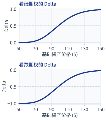
Delta (Δ) 敏感度

  • 定义: Delta 是期权价格 f 相对于基础资产价格 S 的变化率(一阶偏导数): Δ=∂f∂S。
  • 无红利资产的欧式看涨与看跌期权:
    Δcall=N(d1)>0,Δput=N(d1)−1<0
  • Delta 取值范围:
    • 看涨期权 Delta 介于 0 至 +1 之间(平值 ATM≈0.5,深度实值 ITM →1,深度虚值 OTM →0)。
    • 看跌期权 Delta 介于 −1 至 0 之间(平值 ATM≈−0.5,深度实值 ITM →−1,深度虚值 OTM →0)。
看涨期权与看跌期权的 Delta 随基础资产价格变化的曲线
Page 3 · DeltaSlide ↗

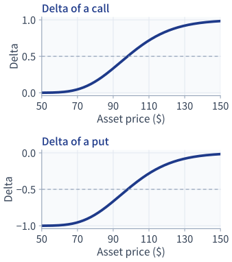
Delta (Δ)

  • Definition: Delta is the rate of change of the option price f with respect to the underlying asset price S: Δ=∂f∂S.
  • European Calls and Puts on Non-Dividend Paying Assets:
    Δcall=N(d1)>0,Δput=N(d1)−1<0
  • Delta Ranges:
    • Call Delta lies between 0 and +1 (ATM≈0.5, deep ITM →1, deep OTM →0).
    • Put Delta lies between −1 and 0 (ATM≈−0.5, deep ITM →−1, deep OTM →0).
Delta of a call and of a put against the asset price
第 4 页 · Delta敏感度幻灯片 ↗

Delta 的核心性质

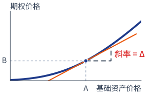
  • 斜率的几何含义: Delta 是期权价格关于基础资产价格 S 曲线上的切线斜率,其中 ΔS、Δf 分别为基础资产价格和期权价格 f 的变化量(符号前的 Δ 表示“变化量”,单独的 Δ 则指期权的 Delta):
    切线斜率=Δ=limΔS→0ΔfΔS
    • 请与上一页的 Delta 曲线对照理解。
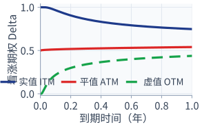
  • Delta 与到期时间的关系:
    • 当到期时间 T→0 时,Delta 曲线在执行价格 K 附近显著变陡:
      • 对于实值看涨期权(S>K):Δ→1.0
      • 对于虚值看涨期权(S<K):Δ→0.0
      • 对于平值看涨期权(S=K):Δ≈0.5,呈现阶跃函数的形态过渡。
期权价格曲线及其切线,切线斜率即 Delta 实值、平值、虚值看涨期权的 Delta 随到期时间的变化
Page 4 · DeltaSlide ↗

Properties of Delta

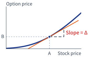
  • Slope Interpretation: Delta is the slope of the curve plotting option price against the underlying asset price S, where ΔS and Δf are the changes in the asset price and in the option price f (here Δ in front of a symbol means "change in", while Δ alone is the option's delta):
    Slope of tangent line=Δ=limΔS→0ΔfΔS
    • Relate this to the previous graphs.
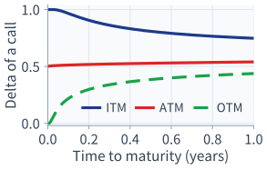
  • Relation between Delta and Time to Maturity:
    • As time to maturity T→0, the delta curve steepens around the strike K:
      • For an ITM call (S>K): Δ→1.0
      • For an OTM call (S<K): Δ→0.0
      • For an ATM call (S=K): Δ≈0.5, transitioning like a step function.
Option price curve with its tangent; the slope of the tangent is Delta Delta of an in-the-money, at-the-money and out-of-the-money call against time to maturity
第 5 页 · Delta敏感度幻灯片 ↗

Delta 的性质(一阶线性近似)

  • Delta 衡量期权价值对基础资产价格微小变动的敏感度:
    • 若资产价格 S 变动 ΔS,则:
      • 看涨期权价值变动约为 Δc×ΔS
      • 看跌期权价值变动约为 Δp×ΔS=−|Δp|×ΔS
  • 数值算例:
    股票价格从 $100 上涨至 $102(ΔS=+$2)。
    该股票看涨期权的 Delta 为 0.5。
    预计该看涨期权价值将上涨: Δ×ΔS=0.5×$2=$1
  • 对于深度实值期权:Δcall≈1,Δput≈−1。
  • 对于深度虚值期权:Δcall≈0,Δput≈0。
Page 5 · DeltaSlide ↗

Properties of Delta (First-Order Linear Approximation)

  • Delta measures the sensitivity of option value to small changes in the underlying asset price:
    • If the underlying price S changes by ΔS, then:
      • Call value changes by approximately Δc×ΔS
      • Put value changes by approximately Δp×ΔS=−|Δp|×ΔS
  • Numerical Example:
    The stock price rises from $100 to $102 (ΔS=+$2).
    A call option on this stock has a delta of 0.5.
    The call value is expected to increase by: Δ×ΔS=0.5×$2=$1
  • For deep ITM options: Δcall≈1,Δput≈−1.
  • For deep OTM options: Δcall≈0,Δput≈0.
第 6 页 · Delta敏感度幻灯片 ↗

远期与期货合约的 Delta

  • 现货资产本身的 Delta 恒为 1。
  • 支付连续红利率 q、期限为 T 的资产远期合约的 Delta:
    Δforward=e−qT(若 q=0⟹Δforward=1)
  • 支付连续红利率 q、期限为 T 的资产期货合约的 Delta:
    Δfutures=e(r−q)T
  • 典型期货实例:
    • 股指期货:Δ=e(r−q)T
    • 外汇期货:Δ=e(r−rf)T(rf 为外国无风险利率)
    • 商品期货(黄金/白银):Δ=erT
Page 6 · DeltaSlide ↗

Delta of Forward and Futures Contracts

  • The delta of the spot contract (underlying asset itself) is 1.
  • The delta of a forward contract with maturity T on an asset paying continuous dividend yield q:
    Δforward=e−qT(if q=0⟹Δforward=1)
  • The delta of a futures contract with maturity T on an asset paying continuous dividend yield q:
    Δfutures=e(r−q)T
  • Examples:
    • Index Futures: Δ=e(r−q)T
    • Currency Futures: Δ=e(r−rf)T (where rf is foreign risk-free rate)
    • Commodity (Gold/Silver) Futures: Δ=erT
第 7 页 · Delta敏感度幻灯片 ↗

期权合约的 Delta

  • 基础资产支付连续红利率 q、期限为 T 的期权,其 Delta:
    Δcall=e−qTN(d1),Δput=e−qT[N(d1)−1]
  • 各类衍生品期权具体形式:
    • 股指期权: Δc=e−qTN(d1),Δp=e−qT[N(d1)−1]
    • 外汇期权: Δc=e−rfTN(d1),Δp=e−rfT[N(d1)−1]
    • 期货期权: Δc=e−rTN(d1),Δp=e−rT[N(d1)−1]
  • 其中代入相应参数计算 d1: d1=ln⁡(S0/K)+(r−q+12σ2)TσT
Page 7 · DeltaSlide ↗

Delta of Option Contracts

  • The delta of an option with maturity T on an asset paying continuous dividend yield q:
    Δcall=e−qTN(d1),Δput=e−qT[N(d1)−1]
  • Examples:
    • Index Options: Δc=e−qTN(d1),Δp=e−qT[N(d1)−1]
    • Currency Options: Δc=e−rfTN(d1),Δp=e−rfT[N(d1)−1]
    • Futures Options: Δc=e−rTN(d1),Δp=e−rT[N(d1)−1]
  • where by choice of q (or rf or r), the appropriate d1 is used: d1=ln⁡(S0/K)+(r−q+12σ2)TσT
第 8 页 · Theta时间衰减幻灯片 ↗

Theta (Θ) 时间衰减

  • 定义: Theta 是期权价格 f 相对于时间流逝 t 的变化率:Θ=∂f∂t。
  • 欧式看涨期权的 Theta:
    Θc=−S0N′(d1)σ2T−rKe−rTN(d2)
    或者,对支付连续红利率 q 的资产:
    Θc=−S0N′(d1)σe−qT2T−rKe−rTN(d2)+qS0N(d1)e−qT
    其中 N′(x)=12πe−x2/2。
  • 期权多头的 Theta 通常为负值 – 随着时间流逝,期权不断损失时间价值。
  • 算例: S0=100,K=100,r=0,σ=0.20,T=1(平值看涨,d1=0.1,N′(0.1)≈0.397): Θ=−100×0.397×0.202=−3.97 / 年 折合 −3.97/252=−0.0158 / 交易日 – 每个交易日约损失 $0.016 的价值。
Page 8 · ThetaSlide ↗

Theta (Θ): Time Decay

  • Definition: Theta is the rate of change of the option price f with respect to the passage of time t: Θ=∂f∂t.
  • Theta of a European call:
    Θc=−S0N′(d1)σ2T−rKe−rTN(d2)
    or, for an asset paying a continuous yield q:
    Θc=−S0N′(d1)σe−qT2T−rKe−rTN(d2)+qS0N(d1)e−qT
    where N′(x)=12πe−x2/2.
  • Theta of a long option position is usually negative – as time passes, the option continually loses time value.
  • Example: S0=100,K=100,r=0,σ=0.20,T=1 (ATM call, d1=0.1, N′(0.1)≈0.397): Θ=−100×0.397×0.202=−3.97 per year Equivalently −3.97/252=−0.0158 per trading day – about $0.016 of value lost per trading day.
第 9 页 · Theta时间衰减幻灯片 ↗

Theta 的性质与特征

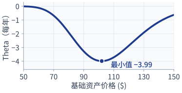
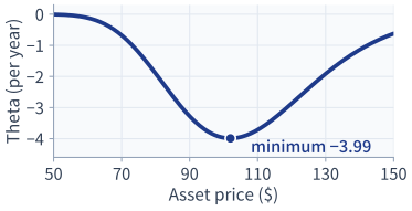
  • Theta 与基础资产价格的关系:
    • 参数设定:K=100,r=0,σ=0.20,T=1。
    • 当期权处于平值状态(ATM,S≈K=100)时,Theta 负值绝对值最大(时间价值损耗速度最快)。
    • 对于深度实值或深度虚值期权,Theta 趋近于 0(因为期权价格被内在价值主导,或者外在时间价值本身极小)。
  • Theta 与到期时间的关系:
    • 对于平值期权,随着到期日临近(T→0),时间衰减急剧加速。
    • 交易员持有临近到期的平值多头期权时,必须警惕严峻的日度时间价值侵蚀。
看涨期权的 Theta 随基础资产价格变化的曲线
Page 9 · ThetaSlide ↗

Properties of Theta

  • Relation between Theta and the underlying asset price:
    • Parameters: K=100,r=0,σ=0.20,T=1.
    • Theta is most negative (time value decays fastest) when the option is at-the-money (ATM,S≈K=100).
    • For deep ITM or deep OTM options, Theta approaches 0 (because the option price is dominated by intrinsic value, or the time value itself is tiny).
  • Relation between Theta and time to maturity:
    • For ATM options, time decay accelerates sharply as expiration approaches (T→0).
    • Traders holding near-expiry ATM long options must watch out for severe daily time-value erosion.
Theta of a call against the asset price
第 10 页 · Gamma曲率幻灯片 ↗

Gamma (Γ) 曲率

  • 定义: Gamma 是 Delta (Δ) 相对于基础资产价格 S 的变化率(期权价格对基础资产价格的二阶偏导数):
    Γ=∂Δ∂S=∂2f∂S2
  • 欧式看涨与看跌期权公式(两者完全相同!):
    Γ=N′(d1)S0σT若含连续红利率 q:Γ=N′(d1)e−qTS0σT
    其中 N′(x)=12πe−x2/2。
  • 若资产价格变动 ΔS,Delta 的变动量约为 Γ×ΔS。
  • 算例: S0=100,K=100,r=0,σ=0.20,T=1,得 Γ≈0.02,Δ≈0.54。
    若股票价格从 $100 上涨至 $110(ΔS=+$10): Δnew≈0.54+(0.02×10)=0.54+0.20=0.74
Page 10 · GammaSlide ↗

Gamma (Γ): Curvature

  • Definition: Gamma is the rate of change of Delta (Δ) with respect to the underlying asset price S (second derivative of the option price with respect to S):
    Γ=∂Δ∂S=∂2f∂S2
  • Formula for European calls and puts (identical for both!):
    Γ=N′(d1)S0σTwith yield q:Γ=N′(d1)e−qTS0σT
    where N′(x)=12πe−x2/2.
  • If the underlying price moves by ΔS, Delta changes by approximately Γ×ΔS.
  • Example: S0=100,K=100,r=0,σ=0.20,T=1, giving Γ≈0.02, Δ≈0.54.
    If the stock price rises from $100 to $110 (ΔS=+$10): Δnew≈0.54+(0.02×10)=0.54+0.20=0.74
第 11 页 · Gamma曲率幻灯片 ↗

Gamma 的性质

  • 虚实值程度对 Gamma 的影响:
    • 深度虚值(Deep OTM): Delta ≈0,随 S 变动极慢 → Γ≈0。
    • 平值状态(ATM): Delta ≈0.5,对资产价格微小变动极度敏感 → Γ 达到峰值最大值!
    • 深度实值(Deep ITM): Delta ≈1.0,随 S 变动极慢 → Γ≈0。
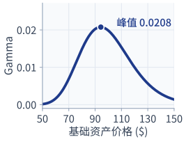
  • Gamma 与基础资产价格的关系:

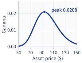
    Gamma 随基础资产价格呈现尖锐的钟形曲线,在执行价格附近(略低于 K)达到峰值。

  • 对冲者必须高度关注持有平值期权的组合,其 Gamma 风险极为集中。
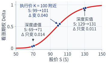
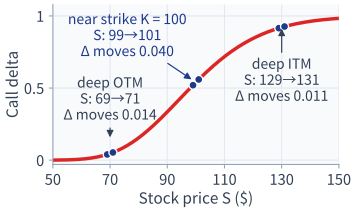
  • 左图:股价同样变动 $2,看涨期权的 Delta 只在执行价 K 附近变化大;右图的 Gamma 就是左图 Delta 曲线的斜率。
看涨期权 Delta 随股价变化的曲线:股价同样变动 $2,深度虚值和深度实值时 Delta 几乎不变,执行价附近变化大 Gamma 随基础资产价格变化的钟形曲线
Page 11 · GammaSlide ↗

Properties of Gamma

  • Moneyness Effect on Gamma:
    • Deep OTM: Delta ≈0, changes very slowly with S → Γ≈0.
    • At-the-Money (ATM): Delta ≈0.5, highly sensitive to small moves in S → Γ reaches its maximum!
    • Deep ITM: Delta ≈1.0, changes very slowly with S → Γ≈0.
  • Relation between Gamma and Asset Price:

    The curve of Gamma against asset price forms a sharp bell-shaped peak close to the strike price (slightly below K).

  • Hedgers must be especially attentive to portfolios with ATM options where Gamma risk is concentrated.
  • Left chart: the same $2 move in the stock price changes the call's delta a lot only near the strike K; Gamma (right chart) is the slope of this delta curve.
Call delta against the stock price: the same $2 move barely changes delta deep out of or deep in the money, but changes it a lot near the strike Gamma against the asset price: a bell-shaped curve
第 12 页 · Gamma曲率幻灯片 ↗

Gamma 的性质与曲率修正

  • Gamma 与到期时间的关系:
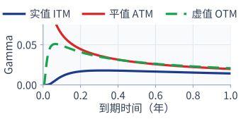
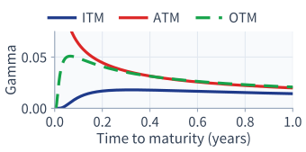
    • 当 T→0 时,平值期权的 Gamma 趋于无穷大,导致在 S=K 附近的敏感度极端集中。
  • Gamma 刻画了 Delta 对冲中的二阶曲率效应:
    • 若 Γ 较小:Delta 变动缓慢 → 较低频率的再平衡即可满足要求。
    • 若 Γ 较大:Delta 高度敏感 → 若不及时调整对冲比例,将引发严重的跟踪误差!
  • 曲率增益直观示例:
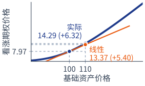
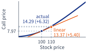
    在 S=100 时,平值看涨期权价格为 $7.97(Δ=0.54,Γ=0.02)。若股票上涨至 $110(ΔS=+10):
    一阶线性 Delta 预测值:7.97+0.54×10=$13.37
    加入 Gamma 修正:13.37+12×0.02×102=13.37+1.00=$14.37
    考虑非线性曲率后的实际看涨期权价格(BSM):$14.29
    约 +$1 的修正项(12ΓΔS2)解释了线性预测 13.37 与实际 14.29 之间的绝大部分差距!
实值、平值、虚值期权的 Gamma 随到期时间的变化 看涨期权价格曲线、Delta 切线的线性预测与实际价格
Page 12 · GammaSlide ↗

Properties of Gamma & Curvature

  • Relation between Gamma and time to maturity:
    • As T→0, ATM Gamma tends to infinity, concentrating extreme sensitivity at S=K.
  • Gamma accounts for curvature in delta hedging:
    • If Γ is small: Delta changes slowly → infrequent rebalancing suffices.
    • If Γ is large: Delta is highly sensitive → leaving the hedge unadjusted causes severe tracking error!
  • Curvature Gain Illustration:
    At S=100, the ATM call is $7.97 (Δ=0.54, Γ=0.02). Stock rises to $110 (ΔS=+10):
    Linear Delta prediction: 7.97+0.54×10=$13.37
    With Gamma correction: 13.37+12×0.02×102=13.37+1.00=$14.37
    Actual call price with curvature (BSM): $14.29
    The ~+$1 correction (12ΓΔS2) explains most of the gap between 13.37 and 14.29!
Gamma of in-the-money, at-the-money and out-of-the-money options against time to maturity Call price curve, the linear (delta) prediction and the actual price
第 13 页 · Delta-Theta-Gamma关系幻灯片 ↗

Delta、Theta 与 Gamma 之间的内在关系

一句话:Delta 对冲只消除股价小幅变动的风险;剩下的是押注股价“大动”还是“不动”。

头寸方向DeltaΓΘ
多头看涨++−
多头看跌−+−
空头看涨−−+
空头看跌+−+

Γ 与 Θ 总是一正一负:对大幅波动的保护(Γ)要用每天的时间损耗(Θ)来付费。

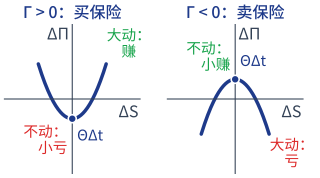
Gamma 为正(买保险)与为负(卖保险)时 ΔΠ 随 ΔS 变化的抛物线

对 Delta 中性组合(组合 Delta =0)的价值变动做泰勒展开:

ΔΠ≈Delta×ΔS⏟=0+ΘΔt+12Γ(ΔS)2

Π 是组合价值(不是希腊字母风险指标)。ΔS、Δt、ΔΠ 里的 Δ 表示“变化量”:股价变动、经过的时间、组合价值变动,不是希腊字母 Delta。组合 Delta 中性,所以第一项为 0。

  • 买入期权并对冲(Γ>0,Θ<0)≈ 买保险:股价不动(ΔS=0)时每天付一点 Θ 损耗;股价大涨或大跌时,Γ 带来的收益超过这笔损耗。
  • 卖出期权并对冲(Γ<0,Θ>0)≈ 卖保险:股价平稳时每天赚取 Θ;一旦股价大幅波动,组合亏损,波动越大亏得越多。
Page 13 · Delta-Theta-GammaSlide ↗

Relationship between Delta, Theta and Gamma

In one line: delta hedging removes only the risk of small moves; what is left is a bet on big moves versus no moves.

PositionDeltaΓΘ
Long Call++−
Long Put−+−
Short Call−−+
Short Put+−+

Γ and Θ always have opposite signs: protection against big moves (Γ) is paid for by daily time decay (Θ).

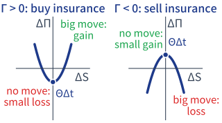
Change in portfolio value against change in asset price: Gamma positive (buying insurance) and Gamma negative (selling insurance)

Taylor expansion for a delta-neutral portfolio (portfolio Delta =0):

ΔΠ≈Delta×ΔS⏟=0+ΘΔt+12Γ(ΔS)2

Π is the portfolio value (not a Greek). The Δ in ΔS, Δt, ΔΠ means “change in”, not the Greek Delta. The portfolio is delta-neutral, so the first term is 0.

  • Buy options and hedge (Γ>0, Θ<0) ≈ buying insurance: no move (ΔS=0): pay a little Θ each day; a big move up or down: the Γ gain exceeds that cost.
  • Sell options and hedge (Γ<0, Θ>0) ≈ selling insurance: quiet days: earn Θ; a big move: a loss, larger the bigger the move.
第 14 页 · Delta-Theta-Gamma关系幻灯片 ↗

简单例子 – 买保险还是卖保险?

设定:1,000 份平值看涨期权,S=K=100, σ=20%, r=0, T=1 年。由 BSM 公式:Γ=0.01985,Θ=−3.97/252=−0.01575 每交易日。买入后用股票做 Delta 对冲(组合 Delta =0)。

一个交易日(Δt=1/252)的盈亏,代入上一页的公式,其中 1,000×ΘΔt=−15.75,1,000×12Γ=9.92:

ΔΠ≈1,000×[ΘΔt+12Γ(ΔS)2]=−15.75+9.92(ΔS)2
当天股价变动 ΔS0±1±2±3
买入并对冲(买保险)−15.75−5.83+23.93+73.53
卖出并对冲(卖保险)+15.75+5.83−23.93−73.53
  • 股价不动:买保险的一方亏 15.75(付了一个交易日的 Θ),卖保险的一方赚 15.75。
  • 盈亏平衡:−15.75+9.92(ΔS)2=0⇒ΔS≈±1.26,正好是一个交易日波动的一个标准差:σSΔt=20%×100×1/252=1.26。
结论:当天股价波动大于一个标准差,买保险的一方赚;小于一个标准差,卖保险的一方赚。这不是巧合:r=0 时 Θ=−12σ2S2Γ,期权价格正好按预期波动定价。
Page 14 · Delta-Theta-GammaSlide ↗

Simple Example – Buying or Selling Insurance?

Setup: 1,000 at-the-money calls, S=K=100, σ=20%, r=0, T=1 year. BSM gives Γ=0.01985 and Θ=−3.97/252=−0.01575 per trading day. Buy them and delta-hedge with the stock.

One trading day (Δt=1/252), from the previous slide, where 1,000×ΘΔt=−15.75 and 1,000×12Γ=9.92:

ΔΠ≈1,000×[ΘΔt+12Γ(ΔS)2]=−15.75+9.92(ΔS)2
Stock move today ΔS0±1±2±3
Buy and hedge (buy insurance)−15.75−5.83+23.93+73.53
Sell and hedge (sell insurance)+15.75+5.83−23.93−73.53
  • No move: the insurance buyer loses 15.75 (a trading day of Θ); the seller earns 15.75.
  • Break-even: −15.75+9.92(ΔS)2=0⇒ΔS≈±1.26=σSΔt, one standard deviation of a trading day's move.
Conclusion: a move bigger than one standard deviation: the buyer wins; smaller: the seller wins. No coincidence: with r=0, Θ=−12σ2S2Γ, so the option is priced for the expected volatility.
第 15 页 · Vega波动率敏感度幻灯片 ↗

Vega (V) 波动率敏感度

  • 定义: Vega 是期权价格 f 相对于基础资产波动率 σ 的变化率: V=∂f∂σ。
  • 欧式看涨与看跌期权公式(两者完全相同):
    V=S0TN′(d1)若含连续红利率 q:V=S0TN′(d1)e−qT
    其中 N′(x)=12πe−x2/2。
  • 无论看涨期权多头还是看跌期权多头,Vega 恒为正值。
  • 经济含义: 若波动率 σ 上升 1%(0.01),期权价格相应上涨约 0.01×V。
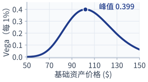
  • Vega 与基础资产价格的关系(见下图):平值期权(ATM)的 Vega 达到最高,随着深入实值或虚值逐渐下降。
Vega 随基础资产价格变化的钟形曲线
Page 15 · VegaSlide ↗

Vega (V)

  • Definition: Vega is the rate of change of option price f with respect to the volatility σ of the underlying asset: V=∂f∂σ.
  • Formula for European Call and Put (identical for both):
    V=S0TN′(d1)or with dividend q:V=S0TN′(d1)e−qT
    where N′(x)=12πe−x2/2.
  • Vega is strictly positive for both long calls and long puts.
  • Interpretation: If volatility σ increases by 1% (0.01), the option price increases by approximately 0.01×V.
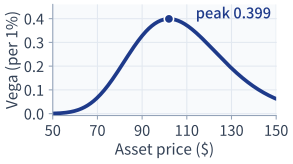
  • Relation between Vega and asset price (chart below): Vega is highest for at-the-money options and drops off for deep ITM/OTM options.
Vega against the asset price: a bell-shaped curve
第 16 页 · Rho利率敏感度幻灯片 ↗

Rho (ρ) 利率敏感度

  • 定义: Rho 是期权价格 f 相对于无风险利率 r 的变化率:
    ρ=∂f∂r
  • 欧式期权计算公式:
    ρcall=KTe−rTN(d2)>0,ρput=−KTe−rTN(−d2)<0
  • 经济含义: 若利率 r 上升 1%(0.01),期权价格相应变动约 0.01×ρ。
  • 外汇期权中的双 Rho 参数:
    • 本国利率 Rho(ρdomestic),衡量对本国无风险利率 r 的敏感度。
    • 外国利率 Rho(ρforeign),衡量对外国无风险利率 rf 的敏感度。
Page 16 · RhoSlide ↗

Rho (ρ)

  • Definition: Rho is the rate of change of option price f with respect to the risk-free interest rate r:
    ρ=∂f∂r
  • Formulas for European Options:
    ρcall=KTe−rTN(d2)>0,ρput=−KTe−rTN(−d2)<0
  • Interpretation: If interest rate r increases by 1% (0.01), option price changes by approximately 0.01×ρ.
  • Currency Options: There are two rho parameters:
    • Domestic Rho (ρdomestic) with respect to domestic rate r.
    • Foreign Rho (ρforeign) with respect to foreign rate rf.
第 17 页 · Rho利率敏感度幻灯片 ↗

交互实验:希腊字母怎么随股价和期限变

默认是前面的算例(S0=K=100,r=0,σ=20%,T=1 年):Gamma ≈ 0.0198,Theta ≈ −3.97 /年。选一个希腊字母,看它在三个期限下随股价的曲线;把 T 调小,Gamma 在 K 附近越来越尖。 新窗口全屏打开 ↗

Page 17 · RhoSlide ↗

Interactive Greeks Explorer

The defaults are the earlier example (S0=K=100, r=0, σ=20%, T=1 year): Gamma ≈ 0.0198, Theta ≈ −3.97 per year. Pick a Greek and see its curve against the stock price for three maturities; shrink T and Gamma gets sharper near K. Open in New Window ↗

第 18 页 · 希腊字母组合管理幻灯片 ↗

希腊字母组合管理:Delta、Gamma 与 Vega 的协同控制

  • 期权投资组合的整体希腊字母是其各个成分合约希腊字母的加权和(组合含 n 个期权,wi 为第 i 个期权的头寸):
    ΔP=∑i=1nwiΔi,ΓP=∑i=1nwiΓi,VP=∑i=1nwiVi
  • 实现 Delta 中性(ΔP=0): 可通过持有现货资产或期货合约达成(现货与期货的 Γ=0,V=0)。
    • 若期货头寸为 wF,现货头寸为 wS:wF=e−(r−q)T∗wS,其中 T∗ 为期货合约的到期日。
  • 实现 Gamma 与 Vega 中性(ΓP=0,VP=0):
    • 现货与期货合约的 Γ 与 V 恒为零。
    • 因此,要调节组合的 Gamma 或 Vega,必须在组合中额外加入场内挂牌的期权合约!
Page 18 · Managing GreeksSlide ↗

Managing Delta, Gamma and Vega

  • The Greek letters of a portfolio of options are weighted sums of the individual Greeks (the portfolio has n options; wi = position in the i-th option):
    ΔP=∑i=1nwiΔi,ΓP=∑i=1nwiΓi,VP=∑i=1nwiVi
  • Delta Neutrality (ΔP=0): Can be achieved using positions in the underlying spot asset or in futures contracts (Γspot=0,Vspot=0).
    • If wF is futures position and wS is spot position: wF=e−(r−q)T∗wS, where T∗ is the maturity of the futures contract.
  • Gamma & Vega Neutrality (ΓP=0,VP=0):
    • The underlying asset and futures have Γ=0 and V=0.
    • Therefore, to alter Gamma or Vega, traded options must be added to the portfolio!
第 19 页 · Delta与Gamma对冲幻灯片 ↗

案例 – Delta 与 Gamma 综合对冲

某金融机构的场外期权组合敏感度为 Δ=−500,Γ=−100。市场上有一只可交易期权:ΔT=0.5,ΓT=0.02。需要多少份期权(w)和多少单位现货(wS)才能同时实现 Gamma 与 Delta 中性?

  • Gamma 与 Delta 中性联立条件(现货的 Γ=0):
    Γ:−100+w×0.02+wS×0=0 Δ:−500+w×0.5+wS×1=0
  • 先解 Gamma:w=1000.02=5,000 份期权;再解 Delta:wS=−(−500+5,000×0.5)=−2,000 单位。
  • 对冲策略: 买入 5,000 份可交易期权,做空 2,000 单位现货。
现货 Γ=0 不影响 Gamma → 先用期权调平 Gamma,再用现货扫尾 Delta。课本原题完整解答见《Hull 习题与解答》第 10 讲。
Page 19 · Delta & Gamma HedgingSlide ↗

Example – Delta and Gamma Hedging

An OTC option portfolio has Δ=−500, Γ=−100. A traded option has ΔT=0.5,ΓT=0.02. Find positions in the option (w) and in units of spot (wS) for joint Gamma and Delta neutrality.

  • Neutrality conditions (spot has Γ=0):
    Γ:−100+w×0.02+wS×0=0 Δ:−500+w×0.5+wS×1=0
  • Gamma gives w=1000.02=5,000 options; Delta then gives wS=−(−500+5,000×0.5)=−2,000 units.
  • Hedge: Buy 5,000 traded options; short 2,000 units of spot.
Spot has Γ=0 → flatten Gamma with the option first, then clear Delta with spot. Original Hull problem with full solution: see Hull Exercises & Solutions, Lecture 10.
第 20 页 · Delta与Gamma对冲幻灯片 ↗

案例 – Delta、Gamma 与 Vega 联合对冲

某场外期权组合的敏感度为 Δ=−200,Γ=−100,V=−120。市场上有两只可交易期权:

  • 期权 1:Δ1=0.5,Γ1=0.02,V1=0.02
  • 期权 2:Δ2=0.1,Γ2=0.01,V2=0.02

设加入期权 1 数量为 w1,期权 2 为 w2,现货为 wS 单位。三维度完全中性要求:

Γ:ΓP+w1Γ1+w2Γ2+wS(0)=0 V:VP+w1V1+w2V2+wS(0)=0 Δ:ΔP+w1Δ1+w2Δ2+wS(1)=0

核心逻辑: 必须先通过两只可交易期权联立求解出满足 Gamma 和 Vega 中性的期权头寸,随后使用现货资产消除剩余 Delta!

Page 20 · Delta & Gamma HedgingSlide ↗

Example – Delta, Gamma and Vega Hedging

An OTC option portfolio has Δ=−200,Γ=−100,V=−120. Two traded options are available:

  • Option 1: Δ1=0.5,Γ1=0.02,V1=0.02
  • Option 2: Δ2=0.1,Γ2=0.01,V2=0.02

Let w1 be the number of option 1 added, w2 of option 2, and wS the units of spot. Full neutrality in all three dimensions requires:

Γ:ΓP+w1Γ1+w2Γ2+wS(0)=0 V:VP+w1V1+w2V2+wS(0)=0 Δ:ΔP+w1Δ1+w2Δ2+wS(1)=0

Key logic: first solve the two traded options simultaneously to achieve Gamma and Vega neutrality, then use the underlying spot asset to eliminate the remaining Delta!

第 21 页 · Delta与Gamma对冲幻灯片 ↗

案例 – Delta、Gamma 与 Vega 对冲(续)

联立线性方程组:

−100+0.02w1+0.01w2=0 −120+0.02w1+0.02w2=0 −200+0.5w1+0.1w2+wS=0
  • 前两式相减:0.01w2=20;回代第一式:0.02w1=100−20=80,即 w2=2,000 份期权 2,w1=4,000 份期权 1
  • 代入 Delta 方程(期权贡献 =2,200): −200+2,200+wS=0⟹wS=−2,000
  • 对冲:买入 4,000 份期权 1、2,000 份期权 2,做空 2,000 单位现货。
  • Delta 中性为微小价格变动提供保护,而 Gamma 中性则在对冲再平衡的时间间隔之间,为大幅价格变动提供保护。
两只期权先联立调平 Γ 与 V,现货再清掉剩余 Delta。课本原题完整解答见《Hull 习题与解答》第 10 讲。
Page 21 · Delta & Gamma HedgingSlide ↗

Example – Delta, Gamma and Vega Hedging (continued)

Solve the simultaneous linear equations:

−100+0.02w1+0.01w2=0 −120+0.02w1+0.02w2=0 −200+0.5w1+0.1w2+wS=0
  • Second minus first: 0.01w2=20; back-substitute: 0.02w1=100−20=80: w2=2,000 of Option 2,w1=4,000 of Option 1
  • Delta equation (options contribute 2,200): −200+2,200+wS=0⟹wS=−2,000
  • Hedge: Buy 4,000 Option 1 and 2,000 Option 2; short 2,000 units.
  • Delta neutrality provides protection against small price moves, while gamma neutrality provides protection against large price moves between hedge rebalancing.
Options flatten Γ and V; spot clears residual Delta. Original Hull problem with full solution: see Hull Exercises & Solutions, Lecture 10.
第 22 页 · 动态对冲实务幻灯片 ↗

实务中的对冲运作 (Hedging in Practice)

  • 日常 Delta 动态对冲: 交易员通常确保其账户头寸每日至少实现一次 Delta 中性(在现代量化交易中,往往利用算法执行进行实时动态微调)。
  • 相机管理 Gamma 与 Vega: 每当市场机会出现且交易成本允许时,交易员会交易场内期权以改善 Gamma 和 Vega 中性程度。
  • 规模经济效应: 随着资产组合规模的扩大,对冲的相对成本显著降低,因为固定交易成本与买卖价差摩擦分摊到了更大的名义交易量上。
Page 22 · Dynamic HedgingSlide ↗

Hedging in Practice

  • Daily Delta Hedging: Traders usually ensure that their books and portfolios are delta-neutral at least once a day (often dynamically rebalanced in real time using algorithmic execution).
  • Opportunistic Gamma and Vega Management: Whenever the opportunity arises and transaction costs allow, traders trade exchange-traded options to improve gamma and vega neutrality.
  • Economies of Scale: As a portfolio becomes larger, hedging becomes relatively less expensive because fixed transaction costs and bid-ask overheads are spread over a much larger notional volume.
第 23 页 · 动态对冲实务幻灯片 ↗

风险对冲的权衡考量:曲率、波动率与再平衡频率

Delta 中性 (Δ=0)
一阶线性保护。 切线拟合。防范微小的价格渐进变动。利用高流动性现货股票或期货易于执行。
Gamma 中性 (Γ=0)
二阶曲率保护。 二次抛物线拟合。防范再平衡间隔期间的价格大幅跳变。消除 Δ 的快速漂移。
Vega 中性 (V=0)
波动率冲击保护。 防范市场突发体制转变与隐含波动率激增(例如金融危机或黑天鹅事件)。

实务中连续对冲与离散对冲的权衡:

  • BSM 理想状态: 零摩擦的连续再平衡可实现完全无风险对冲(ΔΠ=0)。
  • 市场现实: 真实交易中,高频连续再平衡会产生巨大的交易手续费与买卖价差摩擦损耗。
  • 离散跟踪误差: 在离散时间间隔 Δt 内,未对冲的跟踪误差满足:ΔΠ≈12Γ(ΔS)2+ΘΔt+VΔσ。
  • 机构折中策略: 每日利用低成本现货或期货维持 Delta 中性,当挂牌期权具有经济可行性时,阶段性调整对冲 Gamma 与 Vega。
Page 23 · Dynamic HedgingSlide ↗

Risk Management Trade-Offs: Curvature, Volatility & Rebalancing

Delta Neutrality (Δ=0)
First-order protection. Linear tangent fit. Protects against small, incremental price moves. Easily executed with liquid underlying shares or futures.
Gamma Neutrality (Γ=0)
Second-order curvature. Quadratic parabolic fit. Protects against large price jumps between rebalancing intervals. Eliminates rapid drift in Δ.
Vega Neutrality (V=0)
Volatility shock protection. Protects against sudden market regime shifts and implied volatility spikes (e.g. market crashes, COVID crisis).

Continuous vs Discrete Hedging in Practice:

  • The BSM Ideal: Continuous rebalancing with zero friction produces an exact riskless hedge (ΔΠ=0).
  • Market Reality: In real markets, continuous rebalancing incurs prohibitive transaction costs and bid-ask spread friction.
  • Discrete Tracking Error: An unadjusted delta hedge over interval Δt incurs tracking variance: ΔΠ≈12Γ(ΔS)2+ΘΔt+VΔσ.
  • Institutional Compromise: Maintain Delta neutrality daily using low-cost spot or futures contracts, and neutralize Gamma/Vega periodically when liquid exchange-traded options are economically accessible.
第 24 页 · 动态对冲实务幻灯片 ↗

案例 – 欧式看涨期权对冲模拟

数字取最简单的:S0=K=$100,利率 0,不派红利

某金融机构以每份 $2.50 的价格售出了 1,000 份无红利股票的欧式看涨期权(每份对应 1 股),共收到权利金 $2,500。

  • 参数设定: S0=100,K=100,r=0,σ=20%,T=5 周。
  • Black-Scholes 理论价格为每份 $2.47,合计 $2,470;因此该金融机构初始锁定了 $30 的理论利润。
  • 金融机构如何对冲其空头风险?
    1. 裸空头头寸(Naked position): 不采取任何行动。
    2. 备兑头寸(Covered position): 立即全额买入 1,000 股股票。
    3. 止损对冲策略(Stop-loss strategy): 股价涨过 $100 时买入股票,跌破 $100 时卖出股票。
    4. 动态 Delta 对冲(Dynamic delta hedging): 动态调整股票持仓,实时维持 Delta 中性组合。
下面四页逐一比较这四种做法。本例为 Hull 经典对冲案例的简化版,课本原题完整解答见《Hull 习题与解答》第 10 讲。
Page 24 · Dynamic HedgingSlide ↗

Example – Hedging a European Call

Simplest numbers: S0=K=$100, rate 0, no dividends

A financial institution sold 1,000 European calls on a non-dividend-paying stock at $2.50 each (1 share per option), receiving $2,500.

  • Parameters: S0=100,K=100,r=0,σ=20%,T=5 weeks.
  • Black-Scholes price: $2.47 each, $2,470 total; initial theoretical profit: $30.
  • How to hedge the short exposure?
    1. Naked position: Do nothing.
    2. Covered position: Buy 1,000 shares immediately.
    3. Stop-loss strategy: Buy stock above $100; sell below $100.
    4. Dynamic delta hedging: Rebalance the stock holding to stay delta neutral.
The next four slides compare these approaches. Simplified from Hull's classic case. Original Hull problem with full solution: see Hull Exercises & Solutions, Lecture 10.
第 25 页 · 动态对冲实务幻灯片 ↗

裸空头头寸 (Naked Position)

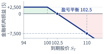
  • 采取裸空头看涨期权时,金融机构不采取任何对冲措施,直接留存初始收取的 $2,500 权利金。
  • 到期损益特征:
    • 若 ST≤100:期权未被行权,金融机构全额保留权利金 =+$2,500。
    • 若 ST>100:期权被对手方行权,金融机构面临无限的上行潜在亏损!
  • 数值示例: 假设 ST=$110:
    损益=(K−ST)×1,000+期权权利金 =($100−$110)×1,000+$2,500=−$7,500
  • 结论: 裸卖空看涨期权使机构暴露于不可控的巨额上行市场风险之中。
裸空头看涨期权的到期损益图
Page 25 · Dynamic HedgingSlide ↗

Naked Position

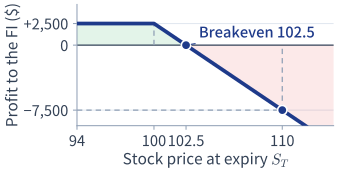
  • With a naked short call, the institution takes no hedging action and simply keeps the initial premium of $2,500.
  • P&L Profile at Expiration:
    • If ST≤100: the option is not exercised and the institution keeps the entire premium =+$2,500.
    • If ST>100: the option is exercised by the counterparty and the institution faces unlimited upside loss potential!
  • Numerical Example: Suppose ST=$110:
    P/L=(K−ST)×1,000+option premium =($100−$110)×1,000+$2,500=−$7,500
  • Conclusion: Writing naked calls exposes the institution to uncontrollable, large upside market risk.
Profit at expiry of a naked short call
第 26 页 · 动态对冲实务幻灯片 ↗

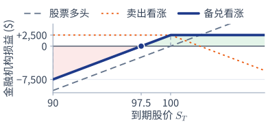
备兑头寸 (Covered Position)

  • 备兑看涨期权策略(Covered Call,见第 7 讲): 卖出 1,000 份看涨期权 + 以 S0=$100 买入 1,000 股股票(初始现金流出 =$100,000)。
  • 损益特征:
    • 若 ST≥100:股票在行权价 K=100 被交割出售,损益 =(100−100)×1,000+$2,500=+$2,500。
    • 若 ST<100:看涨期权虽作废,但所持有的现货股票遭受严重跌价损失!
  • 数值示例: 假设 ST=$90:
    损益=(ST−S0)×1,000+期权权利金 损益=(−$10)×1,000+$2,500=−$7,500
  • 结论: 卖出备兑看涨期权仅仅是将上行风险转换成了严重的下行风险 – 根据买卖权平价定理,这在本质上等价于卖出裸看跌期权!
备兑看涨期权的到期损益图
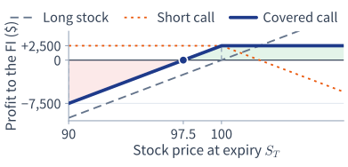
Page 26 · Dynamic HedgingSlide ↗

Covered Position

  • Covered Call Strategy (see Lecture 7): Sell 1,000 call options + buy 1,000 shares at S0=$100 (initial cash outlay =$100,000).
  • P&L Profile:
    • If ST≥100: the stock is delivered and sold at the strike K=100, P/L =(100−100)×1,000+$2,500=+$2,500.
    • If ST<100: the calls expire worthless, but the stock held suffers a severe price loss!
  • Numerical Example: Suppose ST=$90:
    P/L=(ST−S0)×1,000+option premium P/L=(−$10)×1,000+$2,500=−$7,500
  • Conclusion: Writing a covered call merely converts upside risk into severe downside risk – by put-call parity, this is essentially equivalent to writing a naked put!
Profit at expiry of a covered call
第 27 页 · 动态对冲实务幻灯片 ↗

止损对冲策略 (Stop-Loss Strategy)

  • 策略机制:
    • 一旦股票价格突破执行价格 K=$100,立刻买入 1,000 股股票。
    • 一旦股票价格跌破执行价格 K=$100,立刻卖出 1,000 股股票。
  • 理论直觉: 期权在实值时持有股票(形成备兑),期权在虚值时持有现金(避免股票跌价)。
  • 为何在实务中必然失败:
    • 反复拉锯震荡亏损(Whipsaw Losses): 当股票价格在 $100 附近反复震荡时,交易员不断高买($100.10)低卖($99.90)——每来回一次每股亏 $0.20,1,000 股就亏 $200,资金迅速失血!
    • 价格跳空与滑点(Gapping & Slippage): 市场价格跳跃离散,买入和卖出根本无法精确在 $100.00 成交。
    • 货币时间价值: 现金流发生在不同时间点,必须进行折现考量。
Page 27 · Dynamic HedgingSlide ↗

Stop-Loss Strategy

  • Strategy Mechanics:
    • As soon as the stock price rises above the strike K=$100, immediately buy 1,000 shares.
    • As soon as the stock price falls below the strike K=$100, immediately sell 1,000 shares.
  • Theoretical Intuition: Hold the stock when the option is in-the-money (a covered position), and hold cash when it is out-of-the-money (avoiding stock price declines).
  • Why It Is Bound to Fail in Practice:
    • Whipsaw Losses: When the stock price oscillates around $100, the trader keeps buying high ($100.10) and selling low ($99.90) — each round trip loses $0.20 per share, i.e. $200 on 1,000 shares, rapidly bleeding cash!
    • Gapping & Slippage: Market prices jump discretely; purchases and sales cannot be executed at exactly $100.00.
    • Time Value of Money: Cash flows occur at different points in time and must be discounted.
第 28 页 · 动态对冲实务幻灯片 ↗

动态 Delta 对冲 (Dynamic Delta Hedging)

  • BSM 模型的理论基石: 由 Δ 单位基础资产和 1 单位衍生品空头构成的资产组合在局部瞬时是完全无风险的:
    Π=ΔS−f⟹dΠ=rΠdt
  • 其中 Δ 为最优对冲比率:由衍生品价值的变化除以股价的变化计算得出(即期权的 Delta)。
  • 金融机构通过持有 1,000×Δ 股股票来对冲售出 1,000 份看涨期权的空头风险敞口(例如 Δ=0.5 时持有 500 股)。
  • 亦可使用期货合约对冲(见第 16 页):wF=e−(r−q)T∗wS。
  • 为何必须“动态”对冲?
    • 期权 Delta Δ 是资产价格 S 和时间 t 的连续函数。
    • 随着股票价格变动和时间推移,Δ 时刻处于变动之中。
    • 必须定期或连续再平衡持仓,才能维系 Delta 中性状态。
Page 28 · Dynamic HedgingSlide ↗

Dynamic Delta Hedging

  • Theoretical Cornerstone of the BSM Model: A portfolio of Δ units of the underlying asset and 1 short unit of the derivative is locally, instantaneously risk-free:
    Π=ΔS−f⟹dΠ=rΠdt
  • Here Δ is the optimal hedge ratio. It is calculated as the change in value of the derivative divided by the change in stock price (the delta of the option).
  • The institution hedges the short exposure from selling 1,000 calls by holding 1,000×Δ shares (e.g. 500 shares when Δ=0.5).
  • Futures contracts can also be used for delta hedging, see slide 16: wF=e−(r−q)T∗wS.
  • Why Must the Hedge Be “Dynamic”?
    • The option delta Δ is a continuous function of the underlying price S and time t.
    • As the stock price moves and time passes, Δ changes continually.
    • The position must be rebalanced periodically or continuously to maintain delta neutrality.
第 29 页 · 动态对冲实务幻灯片 ↗

案例 – 动态 Delta 对冲模拟 1(到期实值)

卖出 1,000 份看涨(K=100),每周再平衡;r=0 故无利息成本;Delta 取整到 0.1 便于口算
周次股价Delta买入(卖出)股数交易成本 ($)累计成本 ($)
01000.550050,00050,000
1980.4(100)(9,800)40,200
21020.620020,40060,600
31000.5(100)(10,000)50,600
41030.830030,90081,500
51051.020021,000102,500

在第 5 周,期权到期处于实值(S5=105>100)。买方行权:按 K=100 交付 1,000 股,收到 $100,000。
动态对冲净总成本 =$102,500−$100,000=$2,500≈$2,470(理论 BS 价格)。

Page 29 · Dynamic HedgingSlide ↗

Example – Dynamic Delta Hedging Simulation 1 (Expires ITM)

Short 1,000 calls (K=100), rebalanced weekly; r=0, so no interest cost; deltas rounded to 0.1 for easy mental math
WeekStock PriceDeltaShares Bought (Sold)Cost of Shares ($)Cumulative Cost ($)
01000.550050,00050,000
1980.4(100)(9,800)40,200
21020.620020,40060,600
31000.5(100)(10,000)50,600
41030.830030,90081,500
51051.020021,000102,500

In week 5, the option expires in-the-money (S5=105>100). The buyer exercises: 1,000 shares are delivered at K=100, and $100,000 is received.
Net total cost of dynamic hedging =$102,500−$100,000=$2,500≈$2,470 (theoretical BS price).

第 30 页 · 动态对冲实务幻灯片 ↗

案例 – 动态 Delta 对冲模拟 2(到期虚值)

同一笔卖出 1,000 份看涨(K=100),另一条股价路径;r=0,Delta 取整到 0.1
周次股价Delta买入(卖出)股数交易成本 ($)累计成本 ($)
01000.550050,00050,000
11030.610010,30060,300
2980.4(200)(19,600)40,700
31020.510010,20050,900
4990.3(200)(19,800)31,100
5960.0(300)(28,800)2,300

在第 5 周,期权到期处于虚值作废(S5=96<100)。无需交割,持仓已在到期前随 Delta 归零全部卖出。
动态对冲净总成本 =$2,300≈$2,470(理论 BS 价格)。

Page 30 · Dynamic HedgingSlide ↗

Example – Dynamic Delta Hedging Simulation 2 (Expires OTM)

Same sale of 1,000 calls (K=100), but a different stock price path; r=0, deltas rounded to 0.1
WeekStock PriceDeltaShares Bought (Sold)Cost of Shares ($)Cumulative Cost ($)
01000.550050,00050,000
11030.610010,30060,300
2980.4(200)(19,600)40,700
31020.510010,20050,900
4990.3(200)(19,800)31,100
5960.0(300)(28,800)2,300

In week 5, the option expires out-of-the-money and worthless (S5=96<100). No delivery is required; the stock position had already been fully sold off before expiration as Delta went to zero.
Net total cost of dynamic hedging =$2,300≈$2,470 (theoretical BS price).

第 31 页 · 动态对冲实务幻灯片 ↗

交互实验:换一条股价路径,对冲照样有效

同前两页:卖出 1,000 份看涨(S0=K=100,σ=20%,T=5 周,r=0)并做 Delta 对冲。每点一次“新的价格路径”,股价走法都不同,对冲成本却总在 BS 价格附近;改成每天或每小时再平衡,偏差更小。 新窗口全屏打开 ↗

Page 31 · Dynamic HedgingSlide ↗

Interactive Delta Hedging Simulator

Same trade as the previous two pages: sell 1,000 calls (S0=K=100, σ=20%, T=5 weeks, r=0) and delta-hedge them. Each “New price path” moves the stock differently, yet the hedge cost stays near the BS price; rebalancing daily or hourly brings it closer. Open in New Window ↗

第 32 页 · 动态对冲实务幻灯片 ↗

动态对冲与静态对冲的对比分析

  • 动态对冲期权的总成本现值约等于其 Black-Scholes 理论价值(上面两次模拟:$2,500 与 $2,300,均围绕 $2,470 波动,多次模拟的平均值收敛于理论价值)。
  • 动态对冲组合构建了期权的合成多头头寸,从而精确中和了期权卖方的空头敞口。
  • 再平衡频率的权衡: 提高再平衡频率可以降低跟踪误差及对冲成本的波动,但会显著增加累积的交易手续费。
  • 利用远期合约进行静态对冲:
    • 由于远期合约的 Delta 恒等于 1(Δ=1),由 1 股股票多头与 1 份远期合约空头构成的组合完全不需要任何再平衡!
    • 远期合约可以实现“对冲后即可高枕无忧”(静态对冲)。而期权因具有内在非线性曲率,本质上依赖动态 Delta 对冲。
Page 32 · Dynamic HedgingSlide ↗

Dynamic Hedge vs Static Hedge

  • The present value of the total cost of dynamically hedging the option is approximately equal to its Black-Scholes theoretical value (the two simulations above gave $2,500 and $2,300, both scattered around $2,470; averaged over many simulations the cost converges to the theoretical value).
  • The dynamic hedge portfolio creates a synthetic long position in the option, exactly offsetting the option writer's short exposure.
  • Rebalancing Frequency Trade-off: Rebalancing more frequently reduces the tracking error and the variability of hedging cost, but significantly increases cumulative transaction costs.
  • Static Hedging with Forward Contracts:
    • Since a forward contract has a constant delta of 1 (Δ=1), a portfolio of long 1 share of the underlying stock and short 1 forward contract requires no rebalancing at all!
    • Forward contracts allow “hedge and forget” (static hedging). Options, with their inherent nonlinear curvature, inherently rely on dynamic delta hedging.